60分钟入门pytorch

1. Pytorch 是什么Pytorch 是一个基于 Python 的科学计算库，它面向以下两种人群：希望将其代替 Numpy 来利用 GPUs 的威力；一个可以提供更加灵活和快速的深度学习研究平台。1.1 安装略1.2 张量(Tensors)Pytorch 的一大作用就是可以代替 Numpy 库，所以首先介绍 Tensors ，也就是张量，它相当于 Numpy 的多维数组(nd...

GrandNovice

14403人浏览 · 2019-09-15 16:27:21

GrandNovice · 2019-09-15 16:27:21 发布

文章目录

1. Pytorch 是什么
2. autograd
- 2.1 张量
- 2.2 梯度
3. 神经网络
4. 训练分类器
4.1 训练数据
5. 数据并行

1. Pytorch 是什么

Pytorch 是一个基于 Python 的科学计算库，它面向以下两种人群：

希望将其代替 Numpy 来利用 GPUs 的威力；
一个可以提供更加灵活和快速的深度学习研究平台。

1.1 安装

略

1.2 张量(Tensors)

Pytorch 的一大作用就是可以代替 Numpy 库，所以首先介绍 Tensors ，也就是张量，它相当于 Numpy 的多维数组(ndarrays)。两者的区别就是 Tensors 可以应用到 GPU 上加快计算速度。

首先导入必须的库，主要是 torch

from __future__ import print_function
import torch

1.2.1 声明和定义

首先是对 Tensors 的声明和定义方法，分别有以下几种：

torch.empty(): 声明一个未初始化的矩阵。

# 创建一个 5*3 的矩阵
x = torch.empty(5, 3)
print(x)

tensor([[-1.5295e+17,  6.0536e-43, -7.3276e-34],
        [ 6.0536e-43, -1.8921e+17,  6.0536e-43],
        [-7.3276e-34,  6.0536e-43, -1.5295e+17],
        [ 6.0536e-43, -4.4784e-38,  6.0536e-43],
        [-1.8921e+17,  6.0536e-43, -7.3277e-34]])

torch.rand()：随机初始化一个矩阵

# 创建一个随机初始化的 5*3 矩阵
rand_x = torch.rand(5, 3)
print(rand_x)

tensor([[0.1696, 0.8806, 0.9775],
        [0.2274, 0.8217, 0.6517],
        [0.2400, 0.4360, 0.9738],
        [0.6987, 0.4369, 0.4041],
        [0.3466, 0.5234, 0.9666]])

torch.zeros()：创建数值皆为 0 的矩阵

# 创建一个数值皆是 0，类型为 long 的矩阵
zero_x = torch.zeros(5, 3, dtype=torch.long)
print(zero_x)

tensor([[0, 0, 0],
        [0, 0, 0],
        [0, 0, 0],
        [0, 0, 0],
        [0, 0, 0]])

类似的也可以创建数值都是 1 的矩阵，调用 torch.ones

torch.tensor()：直接传递 tensor 数值来创建

# tensor 数值是 [5.5, 3]
tensor1 = torch.tensor([5.5, 3])
print(tensor1)
#tensor0 = torch.tensor([[1,2],[3,4],[5,6]])
#print(tensor0)

tensor([5.5000, 3.0000])

除了上述几种方法，还可以根据已有的 tensor 变量创建新的 tensor 变量，这种做法的好处就是可以保留已有 tensor 的一些属性，包括尺寸大小、数值属性，除非是重新定义这些属性。相应的实现方法如下：

tensor.new_ones(row,cloumn,dtype)：方法需要输入尺寸大小

# 显示定义新的尺寸是 5*3，数值类型是 torch.double
tensor2 = tensor1.new_ones(5, 3, dtype=torch.double)  # new_* 方法需要输入 tensor 大小
print(tensor2)

tensor([[1., 1., 1.],
        [1., 1., 1.],
        [1., 1., 1.],
        [1., 1., 1.],
        [1., 1., 1.]], dtype=torch.float64)

torch.randn_like(old_tensor)：保留相同的尺寸大小

# 修改数值类型
tensor3 = torch.randn_like(tensor2, dtype=torch.float)
print('tensor3: ', tensor3)

tensor3:  tensor([[-1.0496, -0.9908, -0.4547],
        [ 0.6977, -0.9557, -0.8079],
        [ 0.3000,  2.5064,  2.8341],
        [ 1.6385,  0.3932, -1.0152],
        [-1.4500,  1.0717, -0.1984]])

输出结果，这里是根据上个方法声明的 tensor2 变量来声明新的变量，可以看出尺寸大小都是 5*3，但是数值类型是改变了的。

最后，对 tensors 的尺寸大小获取可以采用 tensor.size() 方法：

print(tensor3.size())  
# 输出: torch.Size([5, 3])

torch.Size([5, 3])

注意： torch.Size 实际上是元组(tuple)类型，所以支持所有的元组操作。

1.2.2 操作(Operations)

操作也包含了很多语法，但这里作为快速入门，仅仅以加法操作作为例子进行介绍，更多的操作介绍可以点击下面网址查看官方文档，包括转置、索引、切片、数学计算、线性代数、随机数等等：

https://pytorch.org/docs/stable/torch.html

对于加法的操作，有几种实现方式：

加号（+）运算符
torch.add(tensor1, tensor2, [out=tensor3])，以新的张量tensor3输出
tensor1.add_(tensor2)：直接修改 tensor 变量

tensor4 = torch.rand(5, 3)
print('tensor3 + tensor4= ', tensor3 + tensor4)
print('tensor3 + tensor4= ', torch.add(tensor3, tensor4))
# 新声明一个 tensor 变量保存加法操作的结果
result = torch.empty(5, 3)
torch.add(tensor3, tensor4, out=result)
print('add result= ', result)
# 直接修改变量
tensor3.add_(tensor4)
print('tensor3= ', tensor3)

tensor3 + tensor4=  tensor([[-0.5615, -0.7841, -0.1440],
        [ 1.1251, -0.5450,  0.0642],
        [ 0.4851,  2.8179,  3.4867],
        [ 2.0238,  0.9959, -0.0265],
        [-1.2165,  1.5306,  0.7595]])
tensor3 + tensor4=  tensor([[-0.5615, -0.7841, -0.1440],
        [ 1.1251, -0.5450,  0.0642],
        [ 0.4851,  2.8179,  3.4867],
        [ 2.0238,  0.9959, -0.0265],
        [-1.2165,  1.5306,  0.7595]])
add result=  tensor([[-0.5615, -0.7841, -0.1440],
        [ 1.1251, -0.5450,  0.0642],
        [ 0.4851,  2.8179,  3.4867],
        [ 2.0238,  0.9959, -0.0265],
        [-1.2165,  1.5306,  0.7595]])
tensor3=  tensor([[-0.5615, -0.7841, -0.1440],
        [ 1.1251, -0.5450,  0.0642],
        [ 0.4851,  2.8179,  3.4867],
        [ 2.0238,  0.9959, -0.0265],
        [-1.2165,  1.5306,  0.7595]])

注意：可以改变 tensor 变量的操作都带有一个后缀_, 例如 x.copy_(y), x.t_() 都可以改变 x 变量

除了加法运算操作，对于 Tensor 的访问，和 Numpy 对数组类似，可以使用索引来访问某一维的数据，如下所示：

# 访问 tensor3 第一列数据
print(tensor3[:, 0])

tensor([-0.5615,  1.1251,  0.4851,  2.0238, -1.2165])

对 Tensor 的尺寸修改，可以采用 torch.view() ，如下所示：

x = torch.randn(4, 4)
y = x.view(16)
# -1 表示给定列维度8之后，用16/8=2计算的另一维度数
z = x.view(-1, 8)
print("x = ",x)
print("y = ",y)
print("z = ",z)
print(x.size(), y.size(), z.size())

x =  tensor([[-0.3114,  0.2321,  0.1309, -0.1945],
        [ 0.6532, -0.8361, -2.0412,  1.3622],
        [ 0.7440, -0.2242,  0.6189, -1.0640],
        [-0.1256,  0.6199, -1.5032, -1.0438]])
y =  tensor([-0.3114,  0.2321,  0.1309, -0.1945,  0.6532, -0.8361, -2.0412,  1.3622,
         0.7440, -0.2242,  0.6189, -1.0640, -0.1256,  0.6199, -1.5032, -1.0438])
z =  tensor([[-0.3114,  0.2321,  0.1309, -0.1945,  0.6532, -0.8361, -2.0412,  1.3622],
        [ 0.7440, -0.2242,  0.6189, -1.0640, -0.1256,  0.6199, -1.5032, -1.0438]])
torch.Size([4, 4]) torch.Size([16]) torch.Size([2, 8])

如果 tensor 仅有一个元素，可以采用 .item() 来获取类似 Python 中整数类型的数值：

x = torch.randn(1)
print(x)
print(x.item())
#x1 = torch.rand(1,5)
#print(x1)
#only one element tensors can be converted to Python scalars,所以下面的语句不对
#for x0 in x1.item():
    #print(x0)

tensor([-0.7328])
-0.7328450083732605

更多的运算操作可以查看官方文档的介绍：

https://pytorch.org/docs/stable/torch.html

1.3 和 Numpy 数组的转换

Tensor 和 Numpy 的数组可以相互转换，并且两者转换后共享在 CPU 下的内存空间，即改变其中一个的数值，另一个变量也会随之改变。

1.3.1 Tensor 转换为 Numpy 数组

实现 Tensor 转换为 Numpy 数组的例子如下所示，调用 tensor.numpy() 可以实现这个转换操作。

a = torch.ones(5)
print(a)
b = a.numpy()
print(b)

tensor([1., 1., 1., 1., 1.])
[1. 1. 1. 1. 1.]

此外，刚刚说了两者是共享同个内存空间的，例子如下所示，修改 tensor 变量 a，看看从 a 转换得到的 Numpy 数组变量 b 是否发生变化。

a.add_(1)
print(a)
print(b)

tensor([2., 2., 2., 2., 2.])
[2. 2. 2. 2. 2.]

很明显，b 也随着 a 的改变而改变。

1.3.2 Numpy 数组转换为 Tensor

转换的操作是调用 torch.from_numpy(numpy_array) 方法。例子如下所示：

import numpy as np
a = np.ones(5)
b = torch.from_numpy(a)
np.add(a, 1, out=a)
print(a)
print(b)

[2. 2. 2. 2. 2.]
tensor([2., 2., 2., 2., 2.], dtype=torch.float64)

在 CPU 上，除了 CharTensor 外的所有 Tensor 类型变量，都支持和 Numpy数组的相互转换操作。

1.4. CUDA 张量

Tensors 可以通过 .to 方法转换到不同的设备上，即 CPU 或者 GPU 上。例子如下所示：

# 当 CUDA 可用的时候，可用运行下方这段代码，采用 torch.device() 方法来改变 tensors 是否在 GPU 上进行计算操作
if torch.cuda.is_available():
    device = torch.device("cuda")  # 定义一个 CUDA 设备对象
    y = torch.ones_like(x, device=device)  # 显示创建在 GPU 上的一个 tensor
    x = x.to(device)                       # 也可以采用 .to("cuda") 
    z = x + y
    print(z)
    print(z.to("cpu", torch.double))       # .to() 方法也可以改变数值类型

tensor([0.2672], device='cuda:0')
tensor([0.2672], dtype=torch.float64)

输出结果，第一个结果就是在 GPU 上的结果，打印变量的时候会带有 device=‘cuda:0’，而第二个是在 CPU 上的变量。

本小节教程：

https://pytorch.org/tutorials/beginner/blitz/tensor_tutorial.html

本小节的代码：

https://github.com/ccc013/DeepLearning_Notes/blob/master/Pytorch/practise/basic_practise.ipynb

2. autograd

对于 Pytorch 的神经网络来说，非常关键的一个库就是 autograd ，它主要是提供了对 Tensors 上所有运算操作的自动微分功能，也就是计算梯度的功能。它属于 define-by-run 类型框架，即反向传播操作的定义是根据代码的运行方式，因此每次迭代都可以是不同的。

接下来会简单介绍一些例子来说明这个库的作用。

2.1 张量

torch.Tensor 是 Pytorch 最主要的库，当设置它的属性 .requires_grad=True，那么就会开始追踪在该变量上的所有操作，而完成计算后，可以调用 .backward() 并自动计算所有的梯度，得到的梯度都保存在属性 .grad 中。

调用 .detach() 方法分离出计算的历史，可以停止一个 tensor 变量继续追踪其历史信息，同时也防止未来的计算会被追踪。

而如果是希望防止跟踪历史（以及使用内存），可以将代码块放在 with torch.no_grad(): 内，这个做法在使用一个模型进行评估的时候非常有用，因为模型会包含一些带有 requires_grad=True 的训练参数，但实际上并不需要它们的梯度信息。

对于 autograd 的实现，还有一个类也是非常重要-- Function 。

Tensor 和 Function 两个类是有关联并建立了一个非循环的图，可以编码一个完整的计算记录。每个 tensor 变量都带有属性 .grad_fn ，该属性引用了创建了这个变量的 Function （除了由用户创建的 Tensors，它们的 grad_fn=None )。

如果要进行求导运算，可以调用一个 Tensor 变量的方法 .backward() 。如果该变量是一个标量，即仅有一个元素，那么不需要传递任何参数给方法 .backward()，当包含多个元素的时候，就必须指定一个 gradient 参数，表示匹配尺寸大小的 tensor，这部分见第二小节介绍梯度的内容。

接下来就开始用代码来进一步介绍。

首先导入必须的库：

import torch

开始创建一个 tensor，并让 requires_grad=True 来追踪该变量相关的计算操作：

x = torch.ones(2, 2, requires_grad=True)
print(x)

tensor([[1., 1.],
        [1., 1.]], requires_grad=True)

执行任意计算操作，这里进行简单的加法运算：

y = x + 2
print(y)

tensor([[3., 3.],
        [3., 3.]], grad_fn=<AddBackward0>)

y 是一个操作的结果，所以它带有属性 grad_fn：

print(y.grad_fn)

<AddBackward0 object at 0x000001B088735550>

继续对变量 y 进行操作：

z = y * y * 3
out = z.mean()

print('z=', z)
print('out=', out)

z= tensor([[27., 27.],
        [27., 27.]], grad_fn=<MulBackward0>)
out= tensor(27., grad_fn=<MeanBackward0>)

实际上，一个 Tensor 变量的默认 requires_grad 是 False ，可以像上述定义一个变量时候指定该属性是 True，当然也可以定义变量后，调用 .requires_grad_(True) 设置为 True ，这里带有后缀_ 是会改变变量本身的属性，在上一节介绍加法操作 add_() 说明过，下面是一个代码例子：

#randn函数会因为样本太少而产生较大误差(均值不为0，方差不为1)！！
a = torch.randn(2, 2)
a = ((a * 3) / (a - 1))
#如果有一个单一的输入操作需要梯度，它的输出也需要梯度。相反，只有所有输入都不需要梯度，输出才不需要。
print(a.requires_grad)
a.requires_grad_(True)
print(a.requires_grad)
b = (a * a).sum()
print(b.grad_fn)

False
True
<SumBackward0 object at 0x000001B0887350B8>

第一行是为设置 requires_grad 的结果，接着显示调用 .requires_grad_(True)，输出结果就是 True 。

2.2 梯度

接下来就是开始计算梯度，进行反向传播的操作。out 变量是上一小节中定义的，它是一个标量，因此 out.backward() 相当于 out.backward(torch.tensor(1.)) ，代码如下：

out.backward()
# 输出梯度 d(out)/dx
print(x.grad)

tensor([[4.5000, 4.5000],
        [4.5000, 4.5000]])

结果应该就是得到数值都是 4.5 的矩阵。这里我们用 o 表示 out 变量，那么根据之前的定义会有：

$\frac{1}{4}\sum_iz_i$
$z_i = 3(x_i+2)^2$
$z_i\mid_{x_i=1}=27$

详细来说，初始定义的 x 是一个全为 1 的矩阵，然后加法操作 x+2 得到 y ，接着 y*y*3，得到 z ，并且此时 z 是一个 2*2 的矩阵，所以整体求平均得到 out 变量应该是除以 4，所以得到上述三条公式。

因此，计算梯度：

$\frac{\partial o}{\partial x_i}=\frac{3}{2}(x_i+2)$
$\frac{\partial o}{\partial x_i}\mid_{x_i=1}=\frac{9}{2}=4.5$

从数学上来说，如果你有一个向量值函数：

$\vec y=f(\vec x)$

那么对应的梯度是一个雅克比矩阵(Jacobian matrix)：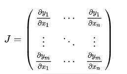
Alt
一般来说，torch.autograd 就是用于计算雅克比向量(vector-Jacobian)乘积的工具。这里略过数学公式，直接上代码例子介绍：

x = torch.randn(3, requires_grad=True)

y = x * 2
while y.data.norm() < 1000: #没太看懂
    y = y * 2

print(y)

输出结果：

tensor([ 237.5009, 1774.2396, 274.0625], grad_fn=< $M u l B a c k w a r d$ >)

这里得到的变量 y 不再是一个标量，torch.autograd 不能直接计算完整的雅克比行列式，但我们可以通过简单的传递向量给 backward() 方法作为参数得到雅克比向量的乘积，例子如下所示：

v = torch.tensor([0.1, 1.0, 0.0001], dtype=torch.float)
y.backward(v)

print(x.grad)

输出结果：

tensor([ 102.4000, 1024.0000, 0.1024])
最后，加上 with torch.no_grad() 就可以停止追踪变量历史进行自动梯度计算：

print(x.requires_grad)
print((x ** 2).requires_grad)

with torch.no_grad():
    print((x ** 2).requires_grad)

输出结果：

True

False
更多有关 autograd 和 Function 的介绍：

https://pytorch.org/docs/autograd

本小节教程：

https://pytorch.org/tutorials/beginner/blitz/autograd_tutorial.html

本小节的代码：

https://github.com/ccc013/DeepLearning_Notes/blob/master/Pytorch/practise/autograd.ipynb

3. 神经网络

在 PyTorch 中 torch.nn 专门用于实现神经网络。其中 nn.Module 包含了网络层的搭建，以及一个方法-- forward(input) ，并返回网络的输出 outptu .

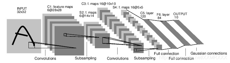
下面是一个经典的 LeNet 网络，用于对字符进行分类。

Alt
对于神经网络来说，一个标准的训练流程是这样的：

1.定义一个多层的神经网络
2.对数据集的预处理并准备作为网络的输入
3.将数据输入到网络
4.计算网络的损失
5.反向传播，计算梯度
6.更新网络的梯度，一个简单的更新规则是 weight = weight - learning_rate * gradient

3.1 定义网络

首先定义一个神经网络，下面是一个 5 层的卷积神经网络，包含两层卷积层和三层全连接层：

import torch
import torch.nn as nn
import torch.nn.functional as F

class Net(nn.Module):

    def __init__(self):
        super(Net, self).__init__()
        # 输入图像是单通道，conv1 kenrnel size=5*5，输出通道 6
        self.conv1 = nn.Conv2d(1, 6, 5)
        # conv2 kernel size=5*5, 输出通道 16
        self.conv2 = nn.Conv2d(6, 16, 5)
        # 全连接层
        self.fc1 = nn.Linear(16*5*5, 120)
        self.fc2 = nn.Linear(120, 84)
        self.fc3 = nn.Linear(84, 10)

    def forward(self, x):
        # max-pooling 采用一个 (2,2) 的滑动窗口
        x = F.max_pool2d(F.relu(self.conv1(x)), (2, 2))
        # 核(kernel)大小是方形的话，可仅定义一个数字，如 (2,2) 用 2 即可
        x = F.max_pool2d(F.relu(self.conv2(x)), 2)
        x = x.view(-1, self.num_flat_features(x))
        x = F.relu(self.fc1(x))
        x = F.relu(self.fc2(x))
        x = self.fc3(x)
        return x

    def num_flat_features(self, x):
        # 除了 batch 维度外的所有维度
        size = x.size()[1:]
        num_features = 1
        for s in size:
            num_features *= s
        return num_features

net = Net()
print(net)

Net(
  (conv1): Conv2d(1, 6, kernel_size=(5, 5), stride=(1, 1))
  (conv2): Conv2d(6, 16, kernel_size=(5, 5), stride=(1, 1))
  (fc1): Linear(in_features=400, out_features=120, bias=True)
  (fc2): Linear(in_features=120, out_features=84, bias=True)
  (fc3): Linear(in_features=84, out_features=10, bias=True)
)

这里必须实现 forward 函数，而 backward 函数在采用 autograd 时就自动定义好了，在 forward 方法可以采用任何的张量操作。

net.parameters() 可以返回网络的训练参数，使用例子如下：

params = list(net.parameters())
print('参数数量: ', len(params))
# conv1.weight
print('第一个参数大小: ', params[0].size())

参数数量:  10
第一个参数大小:  torch.Size([6, 1, 5, 5])

然后简单测试下这个网络，随机生成一个 32*32 的输入：

# 随机定义一个变量输入网络
input = torch.randn(1, 1, 32, 32)
out = net(input)
print(out)

tensor([[ 0.0527,  0.0785, -0.0961, -0.0425,  0.0973,  0.1605, -0.0440, -0.0142,
          0.0985, -0.0596]], grad_fn=<AddmmBackward>)

接着反向传播需要先清空梯度缓存，并反向传播随机梯度：

# 清空所有参数的梯度缓存，然后计算随机梯度进行反向传播
net.zero_grad()
out.backward(torch.randn(1, 10))

注意：

torch.nn 只支持小批量(mini-batches)数据，也就是输入不能是单个样本，比如对于 nn.Conv2d 接收的输入是一个 4 维张量–nSamples * nChannels * Height * Width 。
所以，如果你输入的是单个样本，需要采用 input.unsqueeze(0) 来扩充一个假的 batch 维度，即从 3 维变为 4 维。

3.2 损失函数

损失函数的输入是 (output, target) ，即网络输出和真实标签对的数据，然后返回一个数值表示网络输出和真实标签的差距。

PyTorch 中其实已经定义了不少的损失函数，这里仅采用简单的均方误差：nn.MSELoss ，例子如下：

output = net(input)
# 定义伪标签
target = torch.randn(10)
# 调整大小，使得和 output 一样的 size
target = target.view(1, -1)
criterion = nn.MSELoss()

loss = criterion(output, target)
print(loss)

tensor(0.7520, grad_fn=<MseLossBackward>)

这里，整个网络的数据输入到输出经历的计算图如下所示，其实也就是数据从输入层到输出层，计算 loss 的过程。

input -> conv2d -> relu -> maxpool2d -> conv2d -> relu -> maxpool2d

  -> view -> linear -> relu -> linear -> relu -> linear
  
  -> MSELoss
  
  -> loss

如果调用 loss.backward() ，那么整个图都是可微分的，也就是说包括 loss ，图中的所有张量变量，只要其属性 requires_grad=True ，那么其梯度 .grad张量都会随着梯度一直累计。

用代码来说明：

# MSELoss
print(loss.grad_fn)
# Linear layer
print(loss.grad_fn.next_functions[0][0])
# Relu
print(loss.grad_fn.next_functions[0][0].next_functions[0][0])

<MseLossBackward object at 0x000002830E0584A8>
<AddmmBackward object at 0x000002830E058CF8>
<AccumulateGrad object at 0x000002830E0584A8>

3.3 反向传播

反向传播的实现只需要调用 loss.backward() 即可，当然首先需要清空当前梯度缓存，即.zero_grad() 方法，否则之前的梯度会累加到当前的梯度，这样会影响权值参数的更新。

下面是一个简单的例子，以 conv1 层的偏置参数 bias 在反向传播前后的结果为例：

# 清空所有参数的梯度缓存
net.zero_grad()
print('conv1.bias.grad before backward')
print(net.conv1.bias.grad)

loss.backward()

print('conv1.bias.grad after backward')
print(net.conv1.bias.grad)

conv1.bias.grad before backward
tensor([0., 0., 0., 0., 0., 0.])
conv1.bias.grad after backward
tensor([ 0.0127, -0.0079, -0.0007,  0.0046,  0.0076, -0.0117])

了解更多有关 torch.nn 库，可以查看官方文档：

https://pytorch.org/docs/stable/nn.html

3.4 更新权重

采用随机梯度下降(Stochastic Gradient Descent, SGD)方法的最简单的更新权重规则如下：

weight = weight - learning_rate * gradient

按照这个规则，代码实现如下所示：

# 简单实现权重的更新例子
learning_rate = 0.01
for f in net.parameters():
    f.data.sub_(f.grad.data * learning_rate)

但是这只是最简单的规则，深度学习有很多的优化算法，不仅仅是 SGD，还有 Nesterov-SGD, Adam, RMSProp 等等，为了采用这些不同的方法，这里采用 torch.optim 库，使用例子如下所示：

import torch.optim as optim
# 创建优化器
optimizer = optim.SGD(net.parameters(), lr=0.01)

# 在训练过程中执行下列操作
optimizer.zero_grad() # 清空梯度缓存
output = net(input)
loss = criterion(output, target)
loss.backward()
# 更新权重
optimizer.step()

注意，同样需要调用 optimizer.zero_grad() 方法清空梯度缓存。

本小节教程：

https://pytorch.org/tutorials/beginner/blitz/neural_networks_tutorial.html

本小节的代码：

https://github.com/ccc013/DeepLearning_Notes/blob/master/Pytorch/practise/neural_network.ipynb

4. 训练分类器

上一节介绍了如何构建神经网络、计算 loss 和更新网络的权值参数，接下来需要做的就是实现一个图片分类器。

4.1 训练数据

在训练分类器前，当然需要考虑数据的问题。通常在处理如图片、文本、语音或者视频数据的时候，一般都采用标准的 Python 库将其加载并转成 Numpy 数组，然后再转回为 PyTorch 的张量。

·对于图像，可以采用 Pillow, OpenCV 库；

·对于语音，有 scipy 和 librosa;

·对于文本，可以选择原生 Python 或者 Cython 进行加载数据，或者使用 NLTK 和 SpaCy 。

PyTorch 对于计算机视觉，特别创建了一个 torchvision 的库，它包含一个数据加载器(data loader)，可以加载比较常见的数据集，比如 Imagenet, CIFAR10, MNIST 等等，然后还有一个用于图像的数据转换器(data transformers)，调用的库是 torchvision.datasets 和 torch.utils.data.DataLoader 。

在本教程中，将采用 CIFAR10 数据集，它包含 10 个类别，分别是飞机、汽车、鸟、猫、鹿、狗、青蛙、马、船和卡车。数据集中的图片都是 3x32x32。一些例子如下所示：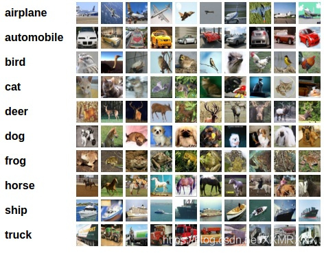
Alt

4.2 训练图片分类器

训练流程如下：

1.通过调用 torchvision 加载和归一化 CIFAR10 训练集和测试集；

2.构建一个卷积神经网络；

3.定义一个损失函数；

4.在训练集上训练网络；

5.在测试集上测试网络性能。

4.2.1 加载和归一化 CIFAR10

首先导入必须的包：

import torch
import torchvision
import torchvision.transforms as transforms

torchvision 的数据集输出的图片都是 PILImage ，即取值范围是 [0, 1] ，这里需要做一个转换，变成取值范围是 [-1, 1] , 代码如下所示：

# 将图片数据从 [0,1] 归一化为 [-1, 1] 的取值范围
transform = transforms.Compose(
    [transforms.ToTensor(),
     transforms.Normalize((0.5, 0.5, 0.5), (0.5, 0.5, 0.5))])

trainset = torchvision.datasets.CIFAR10(root='./data', train=True,
                                        download=True, transform=transform)
trainloader = torch.utils.data.DataLoader(trainset, batch_size=4,
                                          shuffle=True, num_workers=2)

testset = torchvision.datasets.CIFAR10(root='./data', train=False,
                                       download=True, transform=transform)
testloader = torch.utils.data.DataLoader(testset, batch_size=4,
                                         shuffle=False, num_workers=2)

classes = ('plane', 'car', 'bird', 'cat',
           'deer', 'dog', 'frog', 'horse', 'ship', 'truck')

Files already downloaded and verified
Files already downloaded and verified

这里下载好数据后，可以可视化部分训练图片，代码如下：

import matplotlib.pyplot as plt
import numpy as np

# 展示图片的函数
def imshow(img):
    img = img / 2 + 0.5     # 非归一化
    npimg = img.numpy()
    plt.imshow(np.transpose(npimg, (1, 2, 0)))
    plt.show()


# 随机获取训练集图片
dataiter = iter(trainloader)
images, labels = dataiter.next()

# 展示图片
imshow(torchvision.utils.make_grid(images))
# 打印图片类别标签
print(' '.join('%5s' % classes[labels[j]] for j in range(4)))

[外链图片转存失败(img-S87eezU5-1568535314521)(output_38_0.png)]

truck   cat plane horse

展示图片如下所示：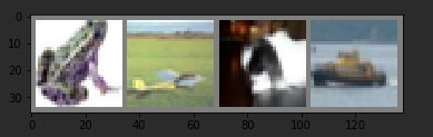
Alt

其类别标签为：

frog plane dog ship

4.2.2 构建一个卷积神经网络

这部分内容其实直接采用上一节定义的网络即可，除了修改 conv1 的输入通道，从 1 变为 3，因为这次接收的是 3 通道的彩色图片。

import torch.nn as nn
import torch.nn.functional as F


class Net(nn.Module):
    def __init__(self):
        super(Net, self).__init__()
        self.conv1 = nn.Conv2d(3, 6, 5)
        self.pool = nn.MaxPool2d(2, 2)
        self.conv2 = nn.Conv2d(6, 16, 5)
        self.fc1 = nn.Linear(16 * 5 * 5, 120)
        self.fc2 = nn.Linear(120, 84)
        self.fc3 = nn.Linear(84, 10)

    def forward(self, x):
        x = self.pool(F.relu(self.conv1(x)))
        x = self.pool(F.relu(self.conv2(x)))
        x = x.view(-1, 16 * 5 * 5)
        x = F.relu(self.fc1(x))
        x = F.relu(self.fc2(x))
        x = self.fc3(x)
        return x


net = Net()

4.2.3 定义损失函数和优化器

这里采用类别交叉熵函数和带有动量的 SGD 优化方法：

import torch.optim as optim

criterion = nn.CrossEntropyLoss()
optimizer = optim.SGD(net.parameters(), lr=0.001, momentum=0.9)

4.2.4 训练网络

第四步自然就是开始训练网络，指定需要迭代的 epoch，然后输入数据，指定次数打印当前网络的信息，比如 loss 或者准确率等性能评价标准。

import time
start = time.time()
for epoch in range(2):

    running_loss = 0.0
    for i, data in enumerate(trainloader, 0):
        # 获取输入数据
        inputs, labels = data
        # 清空梯度缓存
        optimizer.zero_grad()

        outputs = net(inputs)
        loss = criterion(outputs, labels)
        loss.backward()
        optimizer.step()

        # 打印统计信息
        running_loss += loss.item()
        if i % 2000 == 1999:
            # 每 2000 次迭代打印一次信息
            print('[%d, %5d] loss: %.3f' % (epoch + 1, i+1, running_loss / 2000))
            running_loss = 0.0
print('Finished Training! Total cost time in CPU: ', time.time()-start)

[1,  2000] loss: 2.260
[1,  4000] loss: 1.915
[1,  6000] loss: 1.706
[1,  8000] loss: 1.565
[1, 10000] loss: 1.529
[1, 12000] loss: 1.451
[2,  2000] loss: 1.395
[2,  4000] loss: 1.378
[2,  6000] loss: 1.342
[2,  8000] loss: 1.314
[2, 10000] loss: 1.321
[2, 12000] loss: 1.272
Finished Training! Total cost time in CPU:  92.60148167610168

这里定义训练总共 2 个 epoch，训练信息如下，大概耗时为 92s。

4.2.5 测试模型性能

训练好一个网络模型后，就需要用测试集进行测试，检验网络模型的泛化能力。对于图像分类任务来说，一般就是用准确率作为评价标准。

首先，我们先用一个 batch 的图片进行小小测试，这里 batch=4 ，也就是 4 张图片，代码如下：

dataiter = iter(testloader)
images, labels = dataiter.next()

# 打印图片
imshow(torchvision.utils.make_grid(images))
print('GroundTruth: ', ' '.join('%5s' % classes[labels[j]] for j in range(4)))

图片和标签分别如下所示：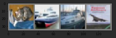
Alt

GroundTruth:    cat  ship  ship plane

然后用这四张图片输入网络，看看网络的预测结果：

# 网络输出
outputs = net(images)

# 预测结果
_, predicted = torch.max(outputs, 1)
print('Predicted: ', ' '.join('%5s' % classes[predicted[j]] for j in range(4)))

Predicted:    cat  ship   car  ship

前面三张图片都预测正确了，第四张图片错误预测飞机为船。

接着，让我们看看在整个测试集上的准确率可以达到多少吧！

correct = 0
total = 0
with torch.no_grad():
    for data in testloader:
        images, labels = data
        outputs = net(images)
        _, predicted = torch.max(outputs.data, 1)
        total += labels.size(0)
        correct += (predicted == labels).sum().item()

print('Accuracy of the network on the 10000 test images: %d %%' % (100 * correct / total))

Accuracy of the network on the 10000 test images: 56 %

这里可能准确率并不一定一样，教程中的结果是 51% ，因为权重初始化问题，可能多少有些浮动，相比随机猜测 10 个类别的准确率(即 10%)，这个结果是不错的，当然实际上是非常不好，不过我们仅仅采用 5 层网络，而且仅仅作为教程的一个示例代码。

然后，还可以再进一步，查看每个类别的分类准确率，跟上述代码有所不同的是，计算准确率部分是 c = (predicted == labels).squeeze()，这段代码其实会根据预测和真实标签是否相等，输出 1 或者 0，表示真或者假，因此在计算当前类别正确预测数量时候直接相加，预测正确自然就是加 1，错误就是加 0，也就是没有变化。

class_correct = list(0. for i in range(10))
class_total = list(0. for i in range(10))
with torch.no_grad():
    for data in testloader:
        images, labels = data
        outputs = net(images)
        _, predicted = torch.max(outputs, 1)
        c = (predicted == labels).squeeze()
        for i in range(4):
            label = labels[i]
            class_correct[label] += c[i].item()
            class_total[label] += 1


for i in range(10):
    print('Accuracy of %5s : %2d %%' % (classes[i], 100 * class_correct[i] / class_total[i]))

Accuracy of plane : 57 %
Accuracy of   car : 60 %
Accuracy of  bird : 40 %
Accuracy of   cat : 34 %
Accuracy of  deer : 38 %
Accuracy of   dog : 52 %
Accuracy of  frog : 70 %
Accuracy of horse : 65 %
Accuracy of  ship : 77 %
Accuracy of truck : 68 %

4.3 在 GPU 上训练

深度学习自然需要 GPU 来加快训练速度的。所以接下来介绍如果是在 GPU 上训练，应该如何实现。

首先，需要检查是否有可用的 GPU 来训练，代码如下：

device = torch.device("cuda:0" if torch.cuda.is_available() else "cpu")
print(device)

cuda:0

输出结果表明你的第一块 GPU 显卡或者唯一的 GPU 显卡是空闲可用状态，否则会打印 cpu 。

既然有可用的 GPU ，接下来就是在 GPU 上进行训练了，其中需要修改的代码如下，分别是需要将网络参数和数据都转移到 GPU 上：

net.to(device)
inputs, labels = inputs.to(device), labels.to(device)

修改后的训练部分代码：

import time
# 在 GPU 上训练注意需要将网络和数据放到 GPU 上
net.to(device)
criterion = nn.CrossEntropyLoss()
optimizer = optim.SGD(net.parameters(), lr=0.001, momentum=0.9)

start = time.time()
for epoch in range(2):

    running_loss = 0.0
    for i, data in enumerate(trainloader, 0):
        # 获取输入数据
        inputs, labels = data
        inputs, labels = inputs.to(device), labels.to(device)
        # 清空梯度缓存
        optimizer.zero_grad()

        outputs = net(inputs)
        loss = criterion(outputs, labels)
        loss.backward()
        optimizer.step()

        # 打印统计信息
        running_loss += loss.item()
        if i % 2000 == 1999:
            # 每 2000 次迭代打印一次信息
            print('[%d, %5d] loss: %.3f' % (epoch + 1, i+1, running_loss / 2000))
            running_loss = 0.0
print('Finished Training! Total cost time in GPU: ', time.time() - start)

[1,  2000] loss: 1.220
[1,  4000] loss: 1.216
[1,  6000] loss: 1.198
[1,  8000] loss: 1.172
[1, 10000] loss: 1.181
[1, 12000] loss: 1.197
[2,  2000] loss: 1.113
[2,  4000] loss: 1.109
[2,  6000] loss: 1.099
[2,  8000] loss: 1.091
[2, 10000] loss: 1.122
[2, 12000] loss: 1.113
Finished Training! Total cost time in GPU:  135.38129496574402

注意，这里调用 net.to(device) 后，需要定义下优化器，即传入的是 CUDA 张量的网络参数。训练结果和之前的类似，而且其实因为这个网络非常小，转移到 GPU 上并不会有多大的速度提升，而且我的训练结果看来反而变慢了，也可能是因为我的笔记本的 GPU 显卡问题。

如果需要进一步提升速度，可以考虑采用多 GPUs，也就是下一节的内容。

本小节教程：

https://pytorch.org/tutorials/beginner/blitz/cifar10_tutorial.html

本小节的代码：

https://github.com/ccc013/DeepLearning_Notes/blob/master/Pytorch/practise/train_classifier_example.ipynb

5. 数据并行

这部分教程将学习如何使用 DataParallel 来使用多个 GPUs 训练网络。

首先，在 GPU 上训练模型的做法很简单，如下代码所示，定义一个 device 对象，然后用 .to() 方法将网络模型参数放到指定的 GPU 上。

这部分教程将学习如何使用 DataParallel 来使用多个 GPUs 训练网络。

首先，在 GPU 上训练模型的做法很简单，如下代码所示，定义一个 device 对象，然后用 .to() 方法将网络模型参数放到指定的 GPU 上。

device = torch.device(“cuda:0”)
model.to(device)

接着就是将所有的张量变量放到 GPU 上：

mytensor = my_tensor.to(device)

注意，这里 my_tensor.to(device) 是返回一个 my_tensor 的新的拷贝对象，而不是直接修改 my_tensor 变量，因此你需要将其赋值给一个新的张量，然后使用这个张量。

Pytorch 默认只会采用一个 GPU，因此需要使用多个 GPU，需要采用 DataParallel ，代码如下所示：

model = nn.DataParallel(model)

这代码也就是本节教程的关键，接下来会继续详细介绍。

5.1 导入和参数

首先导入必须的库以及定义一些参数：

import torch
import torch.nn as nn
from torch.utils.data import Dataset, DataLoader

# Parameters and DataLoaders
input_size = 5
output_size = 2

batch_size = 30
data_size = 100

device = torch.device("cuda:0" if torch.cuda.is_available() else "cpu")

这里主要定义网络输入大小和输出大小，batch 以及图片的大小，并定义了一个 device 对象。

5.2 构建一个假数据集

接着就是构建一个假的(随机)数据集。实现代码如下：

class RandomDataset(Dataset):

    def __init__(self, size, length):
        self.len = length
        self.data = torch.randn(length, size)

    def __getitem__(self, index):
        return self.data[index]

    def __len__(self):
        return self.len

rand_loader = DataLoader(dataset=RandomDataset(input_size, data_size),
                         batch_size=batch_size, shuffle=True)

5.3 简单的模型

接下来构建一个简单的网络模型，仅仅包含一层全连接层的神经网络，加入 print() 函数用于监控网络输入和输出 tensors 的大小：

class Model(nn.Module):
    # Our model

    def __init__(self, input_size, output_size):
        super(Model, self).__init__()
        self.fc = nn.Linear(input_size, output_size)

    def forward(self, input):
        output = self.fc(input)
        print("\tIn Model: input size", input.size(),
              "output size", output.size())

        return output

5.4 创建模型和数据平行

这是本节的核心部分。首先需要定义一个模型实例，并且检查是否拥有多个 GPUs，如果是就可以将模型包裹在 nn.DataParallel ，并调用 model.to(device) 。代码如下：

model = Model(input_size, output_size)
if torch.cuda.device_count() > 1:
  print("Let's use", torch.cuda.device_count(), "GPUs!")
  # dim = 0 [30, xxx] -> [10, ...], [10, ...], [10, ...] on 3 GPUs
  model = nn.DataParallel(model)

model.to(device)

Model(
  (fc): Linear(in_features=5, out_features=2, bias=True)
)

5.5 运行模型

接着就可以运行模型，看看打印的信息：

for data in rand_loader:
    input = data.to(device)
    output = model(input)
    print("Outside: input size", input.size(),
          "output_size", output.size())

	In Model: input size torch.Size([30, 5]) output size torch.Size([30, 2])
Outside: input size torch.Size([30, 5]) output_size torch.Size([30, 2])
	In Model: input size torch.Size([30, 5]) output size torch.Size([30, 2])
Outside: input size torch.Size([30, 5]) output_size torch.Size([30, 2])
	In Model: input size torch.Size([30, 5]) output size torch.Size([30, 2])
Outside: input size torch.Size([30, 5]) output_size torch.Size([30, 2])
	In Model: input size torch.Size([10, 5]) output size torch.Size([10, 2])
Outside: input size torch.Size([10, 5]) output_size torch.Size([10, 2])

5.6 运行结果

如果仅仅只有 1 个或者没有 GPU ，那么 batch=30 的时候，模型会得到输入输出的大小都是 30。但如果有多个 GPUs，那么结果如下：

2 GPUs

# on 2 GPUs
Let’s use 2 GPUs!
In Model: input size torch.Size([15, 5]) output size torch.Size([15, 2])
In Model: input size torch.Size([15, 5]) output size torch.Size([15, 2])
Outside: input size torch.Size([30, 5]) output_size torch.Size([30, 2])
In Model: input size torch.Size([15, 5]) output size torch.Size([15, 2])
In Model: input size torch.Size([15, 5]) output size torch.Size([15, 2])
Outside: input size torch.Size([30, 5]) output_size torch.Size([30, 2])
In Model: input size torch.Size([15, 5]) output size torch.Size([15, 2])
In Model: input size torch.Size([15, 5]) output size torch.Size([15, 2])
Outside: input size torch.Size([30, 5]) output_size torch.Size([30, 2])
In Model: input size torch.Size([5, 5]) output size torch.Size([5, 2])
In Model: input size torch.Size([5, 5]) output size torch.Size([5, 2])
Outside: input size torch.Size([10, 5]) output_size torch.Size([10, 2])

3 GPUs

Let’s use 3 GPUs!
In Model: input size torch.Size([10, 5]) output size torch.Size([10, 2])
In Model: input size torch.Size([10, 5]) output size torch.Size([10, 2])
In Model: input size torch.Size([10, 5]) output size torch.Size([10, 2])
Outside: input size torch.Size([30, 5]) output_size torch.Size([30, 2])
In Model: input size torch.Size([10, 5]) output size torch.Size([10, 2])
In Model: input size torch.Size([10, 5]) output size torch.Size([10, 2])
In Model: input size torch.Size([10, 5]) output size torch.Size([10, 2])
Outside: input size torch.Size([30, 5]) output_size torch.Size([30, 2])
In Model: input size torch.Size([10, 5]) output size torch.Size([10, 2])
In Model: input size torch.Size([10, 5]) output size torch.Size([10, 2])
In Model: input size torch.Size([10, 5]) output size torch.Size([10, 2])
Outside: input size torch.Size([30, 5]) output_size torch.Size([30, 2])
In Model: input size torch.Size([4, 5]) output size torch.Size([4, 2])
In Model: input size torch.Size([4, 5]) output size torch.Size([4, 2])
In Model: input size torch.Size([2, 5]) output size torch.Size([2, 2])
Outside: input size torch.Size([10, 5]) output_size torch.Size([10, 2])

8 GPUs

Let’s use 8 GPUs!
In Model: input size torch.Size([4, 5]) output size torch.Size([4, 2])
In Model: input size torch.Size([4, 5]) output size torch.Size([4, 2])
In Model: input size torch.Size([2, 5]) output size torch.Size([2, 2])
In Model: input size torch.Size([4, 5]) output size torch.Size([4, 2])
In Model: input size torch.Size([4, 5]) output size torch.Size([4, 2])
In Model: input size torch.Size([4, 5]) output size torch.Size([4, 2])
In Model: input size torch.Size([4, 5]) output size torch.Size([4, 2])
In Model: input size torch.Size([4, 5]) output size torch.Size([4, 2])
Outside: input size torch.Size([30, 5]) output_size torch.Size([30, 2])
In Model: input size torch.Size([4, 5]) output size torch.Size([4, 2])
In Model: input size torch.Size([4, 5]) output size torch.Size([4, 2])
In Model: input size torch.Size([4, 5]) output size torch.Size([4, 2])
In Model: input size torch.Size([4, 5]) output size torch.Size([4, 2])
In Model: input size torch.Size([4, 5]) output size torch.Size([4, 2])
In Model: input size torch.Size([4, 5]) output size torch.Size([4, 2])
In Model: input size torch.Size([2, 5]) output size torch.Size([2, 2])
In Model: input size torch.Size([4, 5]) output size torch.Size([4, 2])
Outside: input size torch.Size([30, 5]) output_size torch.Size([30, 2])
In Model: input size torch.Size([4, 5]) output size torch.Size([4, 2])
In Model: input size torch.Size([4, 5]) output size torch.Size([4, 2])
In Model: input size torch.Size([4, 5]) output size torch.Size([4, 2])
In Model: input size torch.Size([4, 5]) output size torch.Size([4, 2])
In Model: input size torch.Size([4, 5]) output size torch.Size([4, 2])
In Model: input size torch.Size([4, 5]) output size torch.Size([4, 2])
In Model: input size torch.Size([4, 5]) output size torch.Size([4, 2])
In Model: input size torch.Size([2, 5]) output size torch.Size([2, 2])
Outside: input size torch.Size([30, 5]) output_size torch.Size([30, 2])
In Model: input size torch.Size([2, 5]) output size torch.Size([2, 2])
In Model: input size torch.Size([2, 5]) output size torch.Size([2, 2])
In Model: input size torch.Size([2, 5]) output size torch.Size([2, 2])
In Model: input size torch.Size([2, 5]) output size torch.Size([2, 2])
In Model: input size torch.Size([2, 5]) output size torch.Size([2, 2])
Outside: input size torch.Size([10, 5]) output_size torch.Size([10, 2])