今天把 “数据加载→模型构建→训练测试” 串成了完整程序，用全连接网络挑战 CIFAR10 分类！过程中踩了不少细节坑，也终于摸清了深度学习训练的核心逻辑～

一、写在前面：拿全连接 “硬刚” 图像任务

明明知道全连接更适合 tabular 数据，但还是想试试：把图像展平成向量，全连接能不能学会分类？ 结果发现 —— 能跑通，但问题不少，模型预测准确率提不上去对于高维度图像全连接还是很吃力，要用到后面的卷积会好很多，刚好暴露了全连接的局限性！

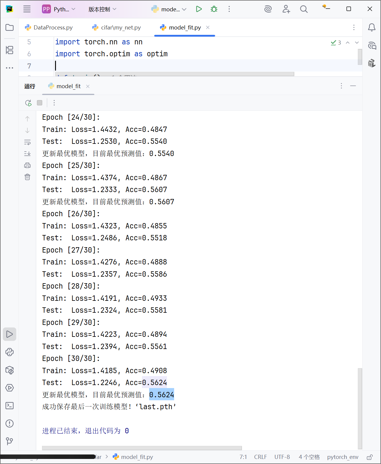
附上训练结果（其实还能通过调参优化结果，不过他的上限就在那，因为比较耗时间咱们不把重点放在这里）：

二、模块 1：数据加载的 “细节战争”

1. 数据集：CIFAR10

• 10 类物体（飞机、汽车…），每张图 3×32×32，是图像分类入门必练数据集。

2. 预处理的 “小心机”

python

# 训练集增强（模拟真实场景）
train_transform = transforms.Compose([
    transforms.RandomCrop(32, padding=4),  # 随机裁剪（先padding再裁，模拟不同视角）
    transforms.RandomHorizontalFlip(p=0.5),  # 50%概率水平翻转
    transforms.ColorJitter(brightness=0.2, contrast=0.2),  # 颜色扰动
    transforms.ToTensor(),  # PIL→Tensor
    transforms.Normalize((0.4914, 0.4822, 0.4465), (0.2023, 0.1994, 0.2010)),  # 归一化
])
​
# 测试集只做基础处理（保持数据真实）
test_transform = transforms.Compose([
    transforms.ToTensor(),
    transforms.Normalize(...),
])

• 训练集增强：通过随机变换，让模型见更多 “变种数据”，增强泛化能力（比如旋转、光照变化的图像）。

• 测试集纯净：只转张量 + 归一化，保证测试结果反映真实能力。

3. 踩坑实录

• 路径错误：一开始 root 写了 "D:\Apps\..."，Windows 下反斜杠会被转义，改成 原始字符串 r"D:\Apps\..." 才解决。

• transform 顺序：必须先做 RandomCrop 等 PIL 操作，再 ToTensor（否则张量无法裁剪）！一开始搞反顺序，报错 “张量没有 size 属性”，debug 了 10 分钟…

三、模块 2：全连接网络的 “线性挣扎”

1. 网络结构设计（4 层全连接 + 正则化）

python

class MyNet(nn.Module):
    def __init__(self, in_features, out_features):
        super().__init__()
        self.model = nn.Sequential(
            # 第一层：512维，加BN、ReLU、Dropout
            nn.Linear(in_features, 512),
            nn.BatchNorm1d(512),  # 加速收敛，稳定训练
            nn.ReLU(),
            nn.Dropout(0.2),  # 随机失活，防过拟合
            
            # 中间层同理...
            
            # 输出层：10类
            nn.Linear(128, out_features),
        )
    
    def forward(self, x):
        x = torch.flatten(x, 1)  # 展平：(batch, 3, 32, 32) → (batch, 3072)
        return self.model(x)

• 为什么加 BatchNorm？ → 让每层输入的分布更稳定，避免 “梯度消失”，训练更快收敛。

• 为什么加 Dropout？ → 训练时随机让 20% 神经元不工作，强迫模型学更鲁棒的特征，测试时恢复所有神经元。

2. 致命缺陷：丢失空间信息

图像是 二维结构（相邻像素有空间关联），但全连接把它展成 一维向量（3×32×32→3072），直接丢失了 “空间关系”（比如边缘、纹理的局部模式）。这就是后续准确率上不去的核心原因！

四、模块 3：训练循环的 “核心逻辑”

1. 关键组件

• 优化器：Adam（自适应调整学习率，比 SGD 更适合复杂任务）。

• 损失函数：CrossEntropyLoss（直接计算类别概率差，分类任务首选）。

• 设备：自动判断 GPU/CPU：

  device = torch.device('cuda' if torch.cuda.is_available() else 'cpu')
  model = MyNet(...).to(device)

2. 训练 vs 测试模式切换

• 训练时：model.train() → 开启 BatchNorm（计算均值 / 方差）和 Dropout（随机失活）。

• 测试时：model.eval() + with torch.no_grad() → 关闭 BatchNorm（用训练好的均值 / 方差）和 Dropout，且不计算梯度（节省内存）。

3. 准确率计算的 “坑”

一开始误把 len(train_data)（batch 数）当样本数，导致准确率超过 100%！正确做法：

python

train_acc = train_acc_total / len(train_data.dataset)  # dataset才是总样本数

五、训练结果反思：全连接的 “天花板”

跑了 30 轮，但测试准确率只有 50% 左右：

• 过拟合：虽然加了 Dropout，但全连接对图像的 “空间信息丢失” 太严重，模型记住了训练集噪声。

• 模型能力不足：无法捕捉图像的局部特征（如边缘、纹理），这些正是 CNN 的强项！

六、今日收获 & 下一步

1. 完整流程闭环：从数据加载、模型构建，到训练测试，终于跑通端到端流程。

2. 认清全连接局限：处理图像时丢失空间信息，为下周学 CNN 埋下强烈动机！

3. 细节决定成败：路径、transform 顺序、准确率计算… 这些小坑，踩过才会印象深刻。

下一步：用 CNN 重新训练 CIFAR10，看看能不能突破准确率瓶颈！

附完整代码：

# 准备数据集

import torch
import torch.nn as nn
from torchvision import datasets,transforms
from torch.utils.data import DataLoader

def train_dataset():

# 创建数据预处理规则

​    transform = transforms.Compose(
        [
         transforms.RandomCrop(32, padding=4),  # 随机裁剪（先pad到36×36，再裁回32×32，模拟不同角度）
         transforms.RandomHorizontalFlip(p=0.5),  # 添加水平翻转（训练时用）
         transforms.ColorJitter(brightness=0.2, contrast=0.2),  # 颜色抖动（亮度/对比度）
         transforms.ToTensor(),
         transforms.Normalize((0.4914, 0.4822, 0.4465), (0.2023, 0.1994, 0.2010)),

​    ]
)

# 创建数据集

dataset = datasets.CIFAR10(
    root='D:\Apps\PyCharm 2025.1.3.1\Demo\Python_PyTorch\data',
    train=True,
    download=False,
    transform=transform
    )

# 加载数据集

train_loader = DataLoader(dataset, batch_size=32, shuffle=True)

return train_loader

def test_dataset():
    transform = transforms.Compose(
        [transforms.ToTensor(),
         transforms.Normalize((0.4914, 0.4822, 0.4465),(0.2023, 0.1994, 0.2010)),
         ]
    )
    dataset = datasets.CIFAR10(
        root = 'D:\Apps\PyCharm 2025.1.3.1\Demo\Python_PyTorch\data',
        train = False,
        download = False,
        transform = transform
    )
    test_loader = DataLoader(dataset, batch_size=32, shuffle=False)
    return test_loader

if __name__ == '__main__':
    train_loader = train_dataset()
    test_loader = test_dataset()
    for x, y in train_loader:
        print(x.shape, y.shape)
        break

for x, y in test_loader:
    print(x.shape, y.shape)
    break

import torch
import torch.nn as nn

# 创建神经网络模型类

class MyNet(nn.Module):
    def __init__(self, in_features, out_features):
        super(MyNet, self).__init__()
        self.model = nn.Sequential(

# 第一层

​           nn.Linear(in_features, 512),
            nn.BatchNorm1d(512),
            nn.ReLU(),
            nn.Dropout(0.2),

# 第二层

​       nn.Linear(512, 256),
        nn.BatchNorm1d(256),
        nn.ReLU(),
        nn.Dropout(0.2),

# 第三层

​       nn.Linear(256, 128),
        nn.BatchNorm1d(128),
        nn.ReLU(),
        nn.Dropout(0.2),

# 输出层

​       nn.Linear(128, out_features),
    )

def forward(self, x):

# 跳过batch维度，展平其他维度

​   x = torch.flatten(x, 1)
    return self.model(x)

if __name__ == '__main__':
    model = MyNet(3*32*32, 10)
    x = torch.randn(4,3,32*32)
    y = model(x)
    print(y.shape)
from DataProcess import train_dataset,test_dataset
from my_net import MyNet

import torch
import torch.nn as nn
import torch.optim as optim

def train():

# 定义使用设备

​   device = torch.device('cuda' if torch.cuda.is_available() else 'cpu')

# 定义模型

​   model = MyNet(3*32*32, 10).to(device)

# 定义数据

​   train_data = train_dataset()
    test_data = test_dataset()



# 定义优化器

optimizer = optim.Adam(model.parameters(),lr = 0.001)# model.parameters()自动调优参数
loss_func = nn.CrossEntropyLoss()# 定义损失函数

# 设置最优模型

best_acc = 0.0

# 开始训练

print('-'*100)
print('开始模型训练！')

epochs = 30
for epoch in range(epochs):

# 每一轮的损失和预测准确率

​   model.train()
    train_loss_total = 0.0
    train_acc_total = 0.0

​   for x, y in train_data:

# 计算预测值

​       x , y = x.to(device), y.to(device)
        y_pred = model(x)

# 计算损失函数

​       loss = loss_func(y_pred, y)

# 开始反向传播

​       optimizer.zero_grad()
        loss.backward()
        optimizer.step()

# 判断类别

# y_pred 的形状是（batch_size,class_num）我们要取所有类别中对应的最大值，就是我们预测的类别

​       y1 = torch.argmax(y_pred, dim=1).to(device)

# 记录每轮结果

​       train_loss_total += loss.item()
        train_acc_total += (y1 == y).sum().item()

# train_loss 计算的是总得损失除以总批次数，他是根据每一批计算一次损失

# train_acc 计算的是所有数据中预测对的数量除以总的数量得到的就是预测准确率

​   train_loss = train_loss_total / len(train_data)
    train_acc = train_acc_total / len(train_data.dataset)

# 进入测试模式

​   model.eval()
    test_acc_total = 0.0
    test_loss_total = 0.0

# 将每次训练好的模型应用到测试集中，判断模型泛化能力

​   with torch.no_grad():# 测试集不参与梯度运算节省内存
        for x, y in test_data:
            x , y = x.to(device), y.to(device)
            y_pred = model(x)
            loss = loss_func(y_pred, y)
            y1 = torch.argmax(y_pred, dim = 1).to(device)

​           test_loss_total += loss.item()
            test_acc_total += (y1 == y).sum().item()

​   test_loss = test_loss_total / len(test_data)
    test_acc = test_acc_total / len(test_data.dataset)

# 打印日志

​   print(f'Epoch [{epoch + 1}/{epochs}]:')
    print(f'Train: Loss={train_loss:.4f}, Acc={train_acc:.4f}')
    print(f'Test:  Loss={test_loss:.4f}, Acc={test_acc:.4f}')

# 保存最优模型

​   if best_acc < test_acc:
        best_acc = test_acc
        torch.save(model.state_dict(), 'best_model.pth')
        print(f'更新最优模型，目前最优预测值：{best_acc:.4f}')

​   if epoch == epochs - 1:
        torch.save(model.state_dict(), 'last.pth')
        print(f'成功保存最后一次训练模型！‘last.pth’')