第一部分：理论理解与问题回答

一、学习与模型（第 1 章）

Q1. 神经网络训练过程中，哪些量是已知的，哪些量是未知的？学习的目标到底是什么？

• 已知量：训练数据集的输入特征（如 MNIST 的像素矩阵）和标签（如数字 0-9 的真实类别）、神经网络的网络结构（层数、每层神经元数）、激活函数 / 损失函数 / 优化器的选择。

• 未知量：权重参数W和偏置参数b

• 学习目标：通过在训练数据上的迭代优化，找到最优的参数(W,b)，使得神经网络未知的测试数据也能做出准确的预测，即实现泛化，让模型的预测输出尽可能接近真实标签，最小化预测误差。

二、线性模型与非线性（第 2 章）

Q2. 为什么单层感知机只能解决线性可分问题？

• 单层感知机的决策边界是线性的，只能处理线性可分的二分类问题，对于非线性问题（如异或门问题），不存在任何超平面能实现完全分隔，因此单层感知机无法解决

Q3. 为什么必须引入非线性激活函数？

• 神经网络的核心目标是拟合现实世界中的非线性复杂规律（如图像、语音、文本的特征映射），而如果仅由线性变换堆叠，无论多少层，最终的整体变换仍为线性变换，无法拟合非线性关系，此时深层网络与单层线性模型没有区别

如果把神经网络中所有激活函数都去掉，会发生什么？

• 任意深度的神经网络退化为单层线性模型，只能解决线性可分问题，无法拟合复杂的非线性数据，失去实际应用价值。

三、神经网络的前向计算（第 3 章）

Q4. 神经网络的前向传播，本质上在做什么数学运算？

• 整个过程是从输入到输出的正向复合映射，核心数学运算为矩阵乘法（实现批量特征的线性变换）和逐元素的非线性运算（激活函数）

Q5. 为什么分类问题中，输出层通常使用 Softmax？

• 分类问题需要模型输出每个类别的概率，且所有类别的概率和为1，方便后续通过概率大小判断预测类别，而Softmax函数恰好满足这一需求

Softmax 在概率意义上做了什么？

• 将无界的logit转换为合法的概率分布，即[0,1]，同时 Softmax 输出的不是绝对概率，而是相对概率

四、损失函数与梯度（第 4 章 · 核心）

Q6. 为什么准确率不能作为训练时的优化目标？

• 准确率是离散的、非可微的函数，而神经网络的训练依赖梯度下降，要求优化目标是连续可微（或分段可微）的函数，只有可微的函数才能计算梯度，进而通过梯度更新参数

为什么必须引入损失函数？

• 损失函数是连续可微的，能计算梯度，为梯度下降提供参数更新的方向；损失函数能精细量化模型的预测误差

五、梯度下降的本质（第 4 章 · 灵魂）

Q7. 梯度在几何意义上代表什么？

• 梯度是损失函数在当前参数点处的方向导数最大值方向，即函数值增长最快的方向，其模长表示该方向上升速率，模长越大，上升越快

为什么沿着负梯度方向更新参数？

• 神经网络的训练目标是最小化损失函数，需要找到损失函数的最小值点。由于梯度方向是上升最快的方向，那么负梯度方向就是损失函数下降最快的方向

Q8. 学习率在梯度下降中起什么作用？

• 学习率η是梯度下降的步长因子，决定了每次沿着负梯度方向更新参数时的步长大小，核心作用是平衡模型的收敛速度和收敛稳定性

学习率过大会怎样？

• 参数更新步长过大，会在损失函数的最小值点附近来回震荡，甚至远离最小值点，导致损失值始终无法下降，模型不收敛

过小又会怎样？

• 参数更新步长过小，需要极多的训练轮次才能接近最小值点，训练效率极低

第二部分：手写神经网络与手写数字识别

要求

任务 1：激活函数

使用 numpy 实现：Sigmoid，ReLU，Softmax

任务 2：损失函数

实现：交叉熵损失（支持 batch 输入）

任务 3：数值梯度

任务 4：实现一个神经网络

任务 5：模型训练

数据集：MNIST

优化方法：SGD

任务 6：实验观察与分析

训练过程中请记录并绘图。

完整代码

# 安装依赖
# pip install numpy matplotlib scikit-learn pandas

# 导入库
import numpy as np
import matplotlib.pyplot as plt
from sklearn.datasets import fetch_openml
from sklearn.model_selection import train_test_split
from sklearn.preprocessing import OneHotEncoder
import time

# 全局设置
plt.rcParams['font.sans-serif'] = ['SimHei']  # 显示中文
plt.rcParams['axes.unicode_minus'] = False  # 显示负号
np.random.seed(42)  # 固定随机种子，保证实验可复现

# 加载MNIST数据集
print("加载MNIST数据集...")
mnist = fetch_openml('mnist_784', version=1, cache=True, as_frame=False)
X = mnist.data
y = mnist.target.astype(np.int32)

# 数据预处理
X = X / 255.0  # 像素归一化到[0,1]，加速训练
X = X.astype(np.float32)

# 标签独热编码（用于交叉熵损失计算）
encoder = OneHotEncoder(sparse_output=False)
y_one_hot = encoder.fit_transform(y.reshape(-1, 1))

# 划分训练集和测试集（60000训练，10000测试）
X_train, X_test, y_train, y_test, y_train_one_hot, y_test_one_hot = train_test_split(
    X, y, y_one_hot, test_size=1 / 7, random_state=42
)

# 查看数据形状
print(f"训练集输入：{X_train.shape}, 训练集标签(独热)：{y_train_one_hot.shape}")
print(f"测试集输入：{X_test.shape}, 测试集标签(独热)：{y_test_one_hot.shape}")


# ===================== 激活函数 =====================
class Activation:
    @staticmethod
    def sigmoid(x):
        """Sigmoid激活函数，带数值稳定性优化"""
        return np.where(x >= 0,
                        1 / (1 + np.exp(-x)),
                        np.exp(x) / (1 + np.exp(x)))

    @staticmethod
    def sigmoid_grad(x):
        """Sigmoid梯度"""
        return Activation.sigmoid(x) * (1 - Activation.sigmoid(x))

    @staticmethod
    def relu(x):
        """ReLU激活函数"""
        return np.maximum(0, x)

    @staticmethod
    def relu_grad(x):
        """ReLU梯度"""
        return np.where(x > 0, 1, 0)

    @staticmethod
    def softmax(x):
        """Softmax激活函数，带数值稳定性优化（防止指数爆炸）"""
        if x.ndim == 2:
            x = x - np.max(x, axis=1, keepdims=True)  # 按行减最大值
            exp_x = np.exp(x)
            return exp_x / np.sum(exp_x, axis=1, keepdims=True)
        else:
            x = x - np.max(x)
            exp_x = np.exp(x)
            return exp_x / np.sum(exp_x)


# ===================== 损失函数 =====================
class Loss:
    @staticmethod
    def cross_entropy_error(y_pred, y_true):
        """
        交叉熵损失，支持batch输入
        :param y_pred: 模型预测的概率分布 (batch_size, n_class)
        :param y_true: 真实标签（独热编码）(batch_size, n_class)
        :return: 批次的平均损失
        """
        if y_pred.ndim == 1:
            y_pred = y_pred.reshape(1, y_pred.size)
            y_true = y_true.reshape(1, y_true.size)

        # 防止log(0)出现，加极小值epsilon
        epsilon = 1e-7
        batch_size = y_pred.shape[0]
        # 仅取真实标签对应的预测概率计算损失
        loss = -np.sum(y_true * np.log(y_pred + epsilon)) / batch_size
        return loss


# 实例化
act = Activation()
loss_fn = Loss()


class TwoLayerNet:
    def __init__(self, input_size, hidden_size, output_size, weight_decay=0.01):
        """
        两层全连接神经网络（输入层→隐藏层→输出层）
        :param input_size: 输入维度（MNIST为784）
        :param hidden_size: 隐藏层神经元数
        :param output_size: 输出维度（MNIST为10）
        :param weight_decay: 权重衰减系数（L2正则化）
        """
        # 初始化参数：He初始化（适用于ReLU）
        self.params = {}
        self.params['W1'] = np.random.randn(input_size, hidden_size) * np.sqrt(2.0 / input_size)
        self.params['b1'] = np.zeros(hidden_size)
        self.params['W2'] = np.random.randn(hidden_size, output_size) * np.sqrt(2.0 / hidden_size)
        self.params['b2'] = np.zeros(output_size)
        self.weight_decay = weight_decay

    def predict(self, x):
        """前向传播，预测概率"""
        W1, W2 = self.params['W1'], self.params['W2']
        b1, b2 = self.params['b1'], self.params['b2']

        # 输入层→隐藏层：线性变换+ReLU
        self.z1 = np.dot(x, W1) + b1
        self.a1 = act.relu(self.z1)
        # 隐藏层→输出层：线性变换+Softmax
        self.z2 = np.dot(self.a1, W2) + b2
        y = act.softmax(self.z2)
        return y

    def loss(self, x, t):
        """计算损失：前向传播+交叉熵+L2正则化"""
        y = self.predict(x)

        # 交叉熵损失
        data_loss = loss_fn.cross_entropy_error(y, t)

        # L2正则化项
        reg_loss = 0.5 * self.weight_decay * (
                np.sum(self.params['W1'] ** 2) + np.sum(self.params['W2'] ** 2)
        )

        return data_loss + reg_loss

    def accuracy(self, x, t):
        """计算准确率（用于评价模型，非优化目标）"""
        y = self.predict(x)
        y_pred = np.argmax(y, axis=1)
        t_true = np.argmax(t, axis=1)
        acc = np.sum(y_pred == t_true) / float(x.shape[0])
        return acc

    def gradient(self, x, t):
        """
        通过反向传播计算梯度
        :param x: 输入数据
        :param t: 真实标签
        :return: 各参数的梯度字典
        """
        batch_size = x.shape[0]

        # 前向传播（确保缓存中间变量）
        y = self.predict(x)

        # 反向传播
        grads = {}

        # 输出层梯度
        dy = (y - t) / batch_size  # Softmax + Cross Entropy的梯度简化形式
        grads['W2'] = np.dot(self.a1.T, dy) + self.weight_decay * self.params['W2']
        grads['b2'] = np.sum(dy, axis=0)

        # 隐藏层梯度
        da1 = np.dot(dy, self.params['W2'].T)
        dz1 = da1 * act.relu_grad(self.z1)
        grads['W1'] = np.dot(x.T, dz1) + self.weight_decay * self.params['W1']
        grads['b1'] = np.sum(dz1, axis=0)

        return grads

    # 保留数值梯度方法用于调试（可选）
    def numerical_gradient(self, x, t):
        """
        计算所有参数的数值梯度（仅用于梯度检查）
        """

        def loss_W(params_dict):
            # 临时保存原始参数
            original_params = self.params.copy()
            # 更新参数
            self.params = params_dict
            # 计算损失
            loss_val = self.loss(x, t)
            # 恢复原始参数
            self.params = original_params
            return loss_val

        grads = {}
        for key in ['W1', 'b1', 'W2', 'b2']:
            grads[key] = self._numerical_gradient_array(loss_W, self.params[key], key)
        return grads

    def _numerical_gradient_array(self, f, x, param_name):
        """辅助函数：计算单个参数的数值梯度"""
        h = 1e-4
        grad = np.zeros_like(x)

        # 对于大矩阵，只采样部分点进行梯度检查
        if x.size > 1000 and param_name.startswith('W'):
            # 随机选择100个位置进行梯度检查
            idx_i = np.random.randint(0, x.shape[0], 100)
            idx_j = np.random.randint(0, x.shape[1], 100)
            for i, j in zip(idx_i, idx_j):
                tmp_val = x[i, j]
                # 计算f(x+h)
                x[i, j] = tmp_val + h
                fxh1 = f(self.params)
                # 计算f(x-h)
                x[i, j] = tmp_val - h
                fxh2 = f(self.params)
                grad[i, j] = (fxh1 - fxh2) / (2 * h)
                # 恢复原始值
                x[i, j] = tmp_val
        else:
            it = np.nditer(x, flags=['multi_index'], op_flags=['readwrite'])
            while not it.finished:
                idx = it.multi_index
                tmp_val = x[idx]
                x[idx] = tmp_val + h
                fxh1 = f(self.params)
                x[idx] = tmp_val - h
                fxh2 = f(self.params)
                grad[idx] = (fxh1 - fxh2) / (2 * h)
                x[idx] = tmp_val
                it.iternext()
        return grad


# 实例化神经网络（MNIST专用）
net = TwoLayerNet(input_size=784, hidden_size=128, output_size=10, weight_decay=0.0001)

# ===================== 训练超参数 =====================
train_epochs = 20  # 训练轮次
batch_size = 128  # 批次大小
lr = 0.1  # 学习率
lr_decay = 0.95  # 学习率衰减
train_size = X_train.shape[0]

# ===================== 训练过程记录 =====================
train_loss_list = []
train_acc_list = []
test_acc_list = []
best_test_acc = 0.0

# 每个轮次的迭代数
iter_per_epoch = max(train_size // batch_size, 1)

# ===================== 开始训练 =====================
print("开始训练神经网络...")
print(f"训练样本数: {train_size}, 批次大小: {batch_size}, 每轮迭代: {iter_per_epoch}")

start_time = time.time()

for epoch in range(train_epochs):
    # 学习率衰减
    current_lr = lr * (lr_decay ** epoch)

    # 随机打乱训练集
    idx = np.random.permutation(train_size)
    X_train_shuffle = X_train[idx]
    y_train_shuffle = y_train_one_hot[idx]

    epoch_loss = 0.0

    for i in range(iter_per_epoch):
        # 采样mini-batch
        start = i * batch_size
        end = min(start + batch_size, train_size)
        x_batch = X_train_shuffle[start:end]
        t_batch = y_train_shuffle[start:end]

        # 计算梯度（使用反向传播）
        grads = net.gradient(x_batch, t_batch)

        # SGD参数更新
        for key in ('W1', 'b1', 'W2', 'b2'):
            net.params[key] -= current_lr * grads[key]

        # 记录训练损失
        loss_val = net.loss(x_batch, t_batch)
        train_loss_list.append(loss_val)
        epoch_loss += loss_val

    # 每个轮次计算一次训练集和测试集的准确率
    train_acc = net.accuracy(X_train[:5000], y_train_one_hot[:5000])  # 用子集加速验证
    test_acc = net.accuracy(X_test[:2000], y_test_one_hot[:2000])  # 用子集加速验证
    train_acc_list.append(train_acc)
    test_acc_list.append(test_acc)

    # 保存最佳模型
    if test_acc > best_test_acc:
        best_test_acc = test_acc
        best_params = net.params.copy()

    # 打印训练日志
    avg_epoch_loss = epoch_loss / iter_per_epoch
    elapsed_time = time.time() - start_time
    print(f"Epoch [{epoch + 1}/{train_epochs}] | "
          f"损失: {avg_epoch_loss:.4f} | "
          f"训练准确率: {train_acc:.4f} | "
          f"测试准确率: {test_acc:.4f} | "
          f"学习率: {current_lr:.4f} | "
          f"用时: {elapsed_time:.1f}s")

# 加载最佳模型
net.params = best_params

# 最终评估（使用全部测试集）
final_train_acc = net.accuracy(X_train[:10000], y_train_one_hot[:10000])
final_test_acc = net.accuracy(X_test, y_test_one_hot)
print(f"\n训练完成！总用时: {time.time() - start_time:.1f}秒")
print(f"最终训练准确率（子集）: {final_train_acc:.4f}")
print(f"最终测试准确率: {final_test_acc:.4f}")

# ===================== 可视化训练结果 =====================
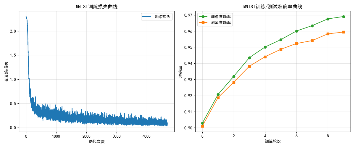
plt.figure(figsize=(15, 5))

# 训练损失曲线
plt.subplot(1, 3, 1)
plt.plot(train_loss_list, label='训练损失', alpha=0.7)
plt.xlabel('迭代次数')
plt.ylabel('交叉熵损失')
plt.title('MNIST训练损失曲线')
plt.legend()
plt.grid(True, alpha=0.3)

# 训练/测试准确率曲线
plt.subplot(1, 3, 2)
x = np.arange(train_epochs)
plt.plot(x, train_acc_list, label='训练准确率', marker='o')
plt.plot(x, test_acc_list, label='测试准确率', marker='s')
plt.xlabel('训练轮次')
plt.ylabel('准确率')
plt.title('MNIST训练/测试准确率曲线')
plt.legend()
plt.grid(True, alpha=0.3)

# 显示一些预测示例
plt.subplot(1, 3, 3)
sample_idx = np.random.choice(len(X_test), 10, replace=False)
sample_images = X_test[sample_idx]
sample_labels = y_test[sample_idx]
sample_pred = np.argmax(net.predict(sample_images), axis=1)

for i in range(10):
    plt.subplot(2, 5, i + 1)
    plt.imshow(sample_images[i].reshape(28, 28), cmap='gray')
    color = 'green' if sample_pred[i] == sample_labels[i] else 'red'
    plt.title(f'真:{sample_labels[i]}\n预:{sample_pred[i]}', color=color, fontsize=8)
    plt.axis('off')

plt.suptitle('MNIST测试集预测示例（绿色=正确，红色=错误）')
plt.tight_layout()
plt.savefig('mnist_train_result.png', dpi=300)
plt.show()


# 梯度检查（可选，验证反向传播正确性）
def gradient_check():
    """梯度检查：比较数值梯度和解析梯度"""
    print("\n执行梯度检查...")

    # 使用小批量数据
    x_check = X_train[:10]
    t_check = y_train_one_hot[:10]

    # 创建临时网络进行梯度检查
    check_net = TwoLayerNet(input_size=784, hidden_size=20, output_size=10, weight_decay=0)

    # 计算解析梯度
    grads_backprop = check_net.gradient(x_check, t_check)

    # 计算数值梯度（只检查部分参数以节省时间）
    grads_numerical = check_net.numerical_gradient(x_check, t_check)

    # 比较差异
    print("梯度检查结果（相对误差）：")
    for key in grads_backprop.keys():
        diff = np.abs(grads_backprop[key] - grads_numerical[key])
        norm = np.abs(grads_backprop[key]) + np.abs(grads_numerical[key]) + 1e-7
        rel_error = np.mean(diff / norm)
        print(f"  {key}: {rel_error:.6f}")

        if rel_error > 1e-4:
            print(f"  警告：{key} 的梯度可能有问题！")

运行结果展示

加载MNIST数据集...
训练集输入：(60000, 784), 训练集标签(独热)：(60000, 10)
测试集输入：(10000, 784), 测试集标签(独热)：(10000, 10)
开始训练神经网络...
训练样本数: 60000, 批次大小: 128, 每轮迭代: 468
Epoch [1/20] | 损失: 0.4345 | 训练准确率: 0.9264 | 测试准确率: 0.9180 | 学习率: 0.1000 | 用时: 3.8s
Epoch [2/20] | 损失: 0.2432 | 训练准确率: 0.9414 | 测试准确率: 0.9325 | 学习率: 0.0950 | 用时: 8.4s
Epoch [3/20] | 损失: 0.2024 | 训练准确率: 0.9514 | 测试准确率: 0.9405 | 学习率: 0.0902 | 用时: 14.2s
Epoch [4/20] | 损失: 0.1753 | 训练准确率: 0.9624 | 测试准确率: 0.9510 | 学习率: 0.0857 | 用时: 18.1s
Epoch [5/20] | 损失: 0.1567 | 训练准确率: 0.9664 | 测试准确率: 0.9505 | 学习率: 0.0815 | 用时: 21.8s
Epoch [6/20] | 损失: 0.1428 | 训练准确率: 0.9682 | 测试准确率: 0.9555 | 学习率: 0.0774 | 用时: 25.4s
Epoch [7/20] | 损失: 0.1318 | 训练准确率: 0.9700 | 测试准确率: 0.9565 | 学习率: 0.0735 | 用时: 29.1s
Epoch [8/20] | 损失: 0.1237 | 训练准确率: 0.9722 | 测试准确率: 0.9590 | 学习率: 0.0698 | 用时: 32.4s
Epoch [9/20] | 损失: 0.1169 | 训练准确率: 0.9742 | 测试准确率: 0.9580 | 学习率: 0.0663 | 用时: 36.0s
Epoch [10/20] | 损失: 0.1112 | 训练准确率: 0.9760 | 测试准确率: 0.9600 | 学习率: 0.0630 | 用时: 39.1s
Epoch [11/20] | 损失: 0.1069 | 训练准确率: 0.9772 | 测试准确率: 0.9610 | 学习率: 0.0599 | 用时: 42.3s
Epoch [12/20] | 损失: 0.1029 | 训练准确率: 0.9794 | 测试准确率: 0.9635 | 学习率: 0.0569 | 用时: 45.9s
Epoch [13/20] | 损失: 0.0997 | 训练准确率: 0.9806 | 测试准确率: 0.9635 | 学习率: 0.0540 | 用时: 49.1s
Epoch [14/20] | 损失: 0.0970 | 训练准确率: 0.9794 | 测试准确率: 0.9655 | 学习率: 0.0513 | 用时: 52.4s
Epoch [15/20] | 损失: 0.0944 | 训练准确率: 0.9814 | 测试准确率: 0.9650 | 学习率: 0.0488 | 用时: 55.6s
Epoch [16/20] | 损失: 0.0921 | 训练准确率: 0.9828 | 测试准确率: 0.9655 | 学习率: 0.0463 | 用时: 58.8s
Epoch [17/20] | 损失: 0.0904 | 训练准确率: 0.9816 | 测试准确率: 0.9665 | 学习率: 0.0440 | 用时: 61.9s
Epoch [18/20] | 损失: 0.0887 | 训练准确率: 0.9840 | 测试准确率: 0.9685 | 学习率: 0.0418 | 用时: 65.2s
Epoch [19/20] | 损失: 0.0870 | 训练准确率: 0.9844 | 测试准确率: 0.9660 | 学习率: 0.0397 | 用时: 68.4s
Epoch [20/20] | 损失: 0.0858 | 训练准确率: 0.9826 | 测试准确率: 0.9690 | 学习率: 0.0377 | 用时: 71.6s

训练完成！总用时: 71.8秒
最终训练准确率（子集）: 0.9817
最终测试准确率: 0.9687

实验记录