卷积原理

卷积核不停的在原图上进行滑动，对应元素相乘再相加。

下图为每次滑动移动1格，然后再利用原图与卷积核上的数值进行计算得到缩略图矩阵的数据，如下图右所示。

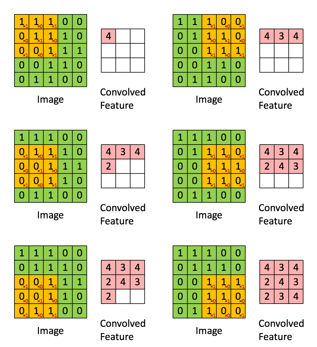
示例如图

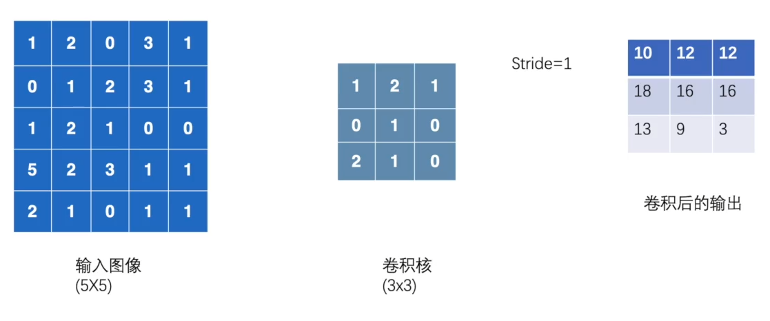
input输入格式：tensor类型（minibatch，in_channels，iH，iW）（最小批次，通道数，高度，宽度）

输入要进行卷积操作的5*5二维矩阵

input = torch.tensor([[1, 2, 0, 3, 1],
                      [0, 1, 2, 3, 1],
                      [1, 2, 1, 0, 0],
                      [5, 2, 3, 1, 1],
                      [2, 1, 0, 1, 1]])

设定3*3的卷积核kernel

kernel = torch.tensor([[1, 2, 1],
                       [0, 1, 0],
                       [2, 1, 0]])

查看输入矩阵和卷积核尺寸

print(input.shape)
print(kernel.shape)

得到大小为5*5和3*3，不符合输入的尺寸要求

尺寸变换的方法

input = torch.reshape(input,(1,1,5,5))
kernel = torch.reshape(kernel,(1,1,3,3))

再次查看尺寸

将包名设定为F

import torch.nn.functional as F

调用conv2d进行卷积操作，步长为1，并输出结果

output = F.conv2d(input,kernel,stride=1)
print(output)

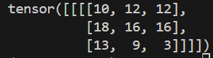
结果为

步长为2时

output2 = F.conv2d(input,kernel,stride=2)
print(output2)

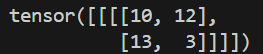
结果为

完整代码

import torch
import torch.nn.functional as F
from nn_module import output

input = torch.tensor([[1, 2, 0, 3, 1],
                      [0, 1, 2, 3, 1],
                      [1, 2, 1, 0, 0],
                      [5, 2, 3, 1, 1],
                      [2, 1, 0, 1, 1]])

kernel = torch.tensor([[1, 2, 1],
                       [0, 1, 0],
                       [2, 1, 0]])

input = torch.reshape(input,(1,1,5,5))
kernel = torch.reshape(kernel,(1,1,3,3))

print(input.shape)
print(kernel.shape)

output = F.conv2d(input,kernel,stride=1)
print(output)

output2 = F.conv2d(input,kernel,stride=2)
print(output2)

步幅、填充原理

步幅（Stride）：卷积核经过输入特征图的采样间隔。设置步幅的目的：希望减小输入参数的数目，减少计算量。

填充：在输入特征图的每一边添加一定数目的行列。设置填充的目的：希望每个输入方块都能作为卷积窗口的中心，或使得输出的特征图的长、宽 = 输入的特征图的长、宽。

一个尺寸 a * a 的特征图，经过 b * b 的卷积层，步幅（stride）= c，填充（padding）= d，若d等于0，也就是不填充，输出的特征图的尺寸 =（a-b）/ c+1；若d不等于0，也就是填充，输出的特征图的尺寸 =（a+2d-b）/ c+1。

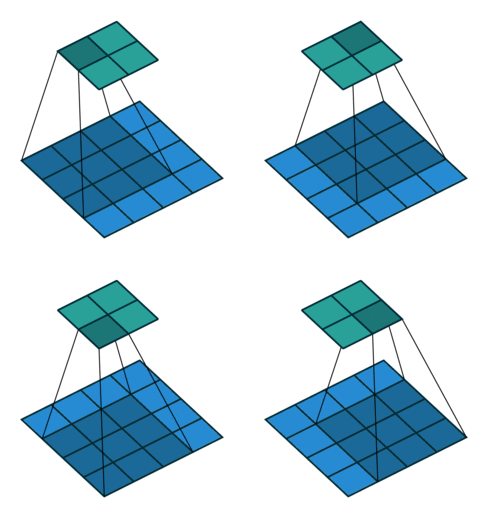
例子1：一个特征图尺寸为4 * 4的输入，使用3 * 3的卷积核，步幅=1，填充=0，输出的尺寸=(4 - 3)/1 + 1 = 2。

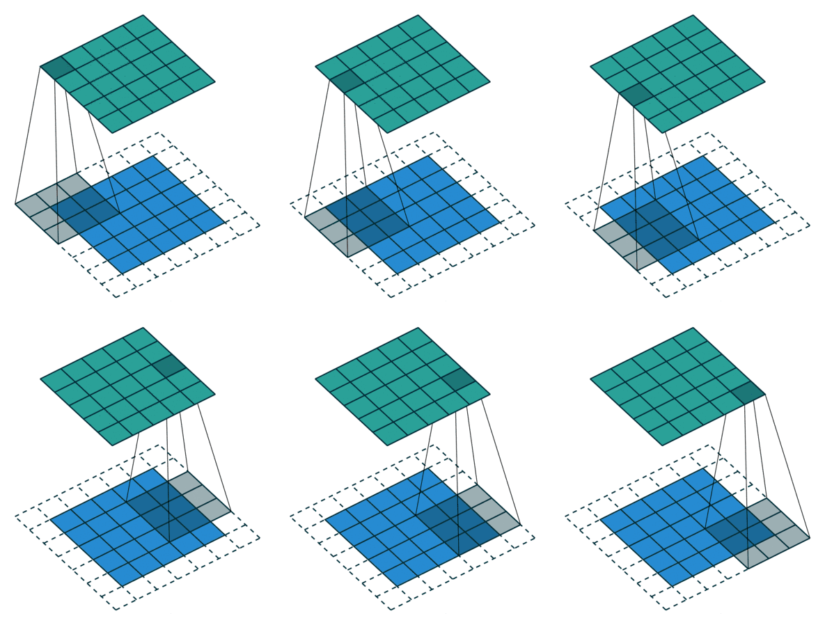
例子2：  一个特征图尺寸为5 * 5的输入，使用3 * 3的卷积核，步幅=1，填充=1，输出的尺寸=(5 + 2 * 1 - 3)/1 + 1 = 5。

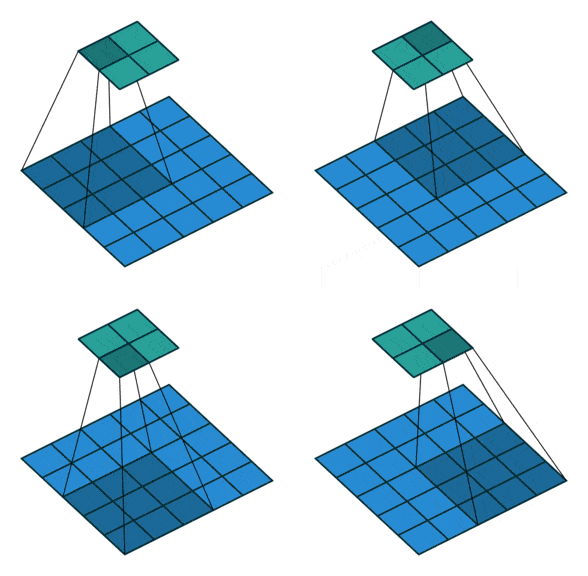
例子3：一个特征图尺寸为5 * 5的输入， 使用3 * 3的卷积核，步幅=2，填充=0，输出的尺寸=(5-3)/2 + 1 = 2。

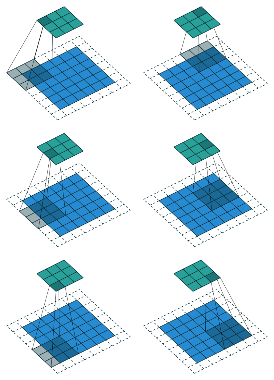
例子4：一个特征图尺寸为6 * 6的输入， 使用3 * 3的卷积核，步幅=2，填充=1，输出的尺寸=(6 + 2 * 1 - 3)/2 + 1 = 2.5 + 1 = 3.5 向下取整=3（降采样：边长减少1/2）。