
【深度学习|Diffusion Model】(二) 奠基之作DDPM详解
前言
在扩散模型的学习过程中,up主deep_thoughts的视频给了我很大的帮助,下面是我在学习过程中观看的一些视频,大家也可以按照这个顺序进行学习。DDPM论文链接也在此给大家列出:https://arxiv.org/abs/2006.11239
up主deep_thoughts
————————
54 DDPM 原来讲解和demo代码演示
58 借助IDDPM代码讲解DDPM
64 DDIM原理和代码
————————
62 分数扩散模型一
63 分数扩散模型二
————————
66 Guided Diffusion
注:本文章难度较大,篇幅较长,大家在阅读过程中需要一些耐心!
一、前置数学知识
在学习DDPM原理之前,了解一些数学概率论的知识是必要的,因为在DDPM中涉及到很多概率公式的推导。
1、先验概率和后验概率
先验概率:根据以往经验和分析得到的概率,它往往作为“由因求果”问题中的“因”出现,如
q
(
x
t
∣
x
t
−
1
)
q(x_t|x_{t-1})
q(xt∣xt−1)
后验概率:指在得到“结果”的信息后重新修正的概率,是“执果寻因”问题中的“因", 如
p
(
x
t
−
1
∣
x
t
)
p(x_{t-1}|x_t)
p(xt−1∣xt)
2、条件概率
设A、B为任意两个事件,若P(A)>0,称在已知事件A发生的条件下,事件B发生的概率为条件概率,记为
P
(
B
∣
A
)
P(B|A)
P(B∣A)
P
(
B
∣
A
)
=
P
(
A
,
B
)
P
(
A
)
P(B|A)=\frac{P(A,B)} {P(A)}
P(B∣A)=P(A)P(A,B)
3、乘法公式:
P
(
A
,
B
)
=
P
(
B
∣
A
)
P
(
A
)
P(A,B)=P(B|A)P(A)
P(A,B)=P(B∣A)P(A)
4、乘法公式一般形式:
P
(
A
,
B
,
C
)
=
P
(
C
∣
B
,
A
)
P
(
B
,
A
)
=
P
(
C
∣
B
,
A
)
P
(
B
∣
A
)
P
(
A
)
P(A,B,C)=P(C|B,A)P(B,A)=P(C|B,A)P(B|A)P(A)
P(A,B,C)=P(C∣B,A)P(B,A)=P(C∣B,A)P(B∣A)P(A)
5、贝叶斯公式:
P
(
A
∣
B
)
=
P
(
B
∣
A
)
P
(
A
)
P
(
B
)
P(A|B)=\frac{P(B|A)P(A)}{P(B)}
P(A∣B)=P(B)P(B∣A)P(A)
6、多元贝叶斯公式:
P
(
A
∣
B
,
C
)
=
P
(
A
,
B
,
C
)
P
(
B
,
C
)
=
P
(
B
∣
A
,
C
)
P
(
A
,
C
)
P
(
B
,
C
)
=
P
(
B
∣
A
,
C
)
P
(
A
∣
C
)
P
(
C
)
P
(
B
∣
C
)
P
(
C
)
=
P
(
B
∣
A
,
C
)
P
(
A
∣
C
)
)
P
(
B
∣
C
)
P(A|B,C)=\frac{P(A,B,C)}{P(B,C)}=\frac{P(B|A,C)P(A,C)}{P(B,C)}=\frac{P(B|A,C)P(A|C)P(C)}{P(B|C)P(C)}=\frac{P(B|A,C)P(A|C))}{P(B|C)}
P(A∣B,C)=P(B,C)P(A,B,C)=P(B,C)P(B∣A,C)P(A,C)=P(B∣C)P(C)P(B∣A,C)P(A∣C)P(C)=P(B∣C)P(B∣A,C)P(A∣C))
7、正态分布的叠加性:
当有两个独立的正态分布变量
N
1
N_{1}
N1和
N
2
N_{2}
N2,它们的均值和方差分别为
μ
1
,
μ
2
\mu_{1},\mu_{2}
μ1,μ2和
σ
1
2
,
σ
2
2
\sigma_{1}^2,\sigma_{2}^2
σ12,σ22它们的和为
N
=
a
N
1
+
b
N
2
N=a N_{1}+b N_{2}
N=aN1+bN2的均值和方差可以表示如下:
E
(
N
)
=
E
(
a
N
1
+
b
N
2
)
=
a
μ
1
+
b
μ
2
V
a
r
(
N
)
=
V
a
r
(
a
N
1
+
b
N
2
)
=
a
2
σ
1
2
+
b
2
σ
2
2
E(N)=E(aN_{1}+bN_{2})=a\mu_{1}+b\mu_{2}\\ Var(N)=Var(aN_{1}+bN_{2})=a^2\sigma_{1}^2+b^2\sigma_{2}^2
E(N)=E(aN1+bN2)=aμ1+bμ2Var(N)=Var(aN1+bN2)=a2σ12+b2σ22
相减时:
E
(
N
)
=
E
(
a
N
1
−
b
N
2
)
=
a
μ
1
−
b
μ
2
V
a
r
(
N
)
=
V
a
r
(
a
N
1
−
b
N
2
)
=
a
2
σ
1
2
+
b
2
σ
2
2
E(N)=E(aN_{1}-bN_{2})=a\mu_{1}-b\mu_{2}\\ Var(N)=Var(aN_{1}-bN_{2})=a^2\sigma_{1}^2+b^2\sigma_{2}^2
E(N)=E(aN1−bN2)=aμ1−bμ2Var(N)=Var(aN1−bN2)=a2σ12+b2σ22
8、参数重整化(重参数化):
若希望从高斯分布
N
(
μ
,
σ
)
N(\mu,\sigma)
N(μ,σ)中采样,可以先从标准分布
N
(
0
,
1
)
N(0,1)
N(0,1)采样出
z
z
z,再得到
σ
∗
z
+
μ
\sigma*z+\mu
σ∗z+μ,这样做的好处是将随机性转移到
z
z
z这个常量上,而
σ
\sigma
σ和
μ
\mu
μ则当做仿射变换网络的一部分。
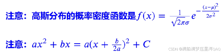
9、高斯分布的概率密度函数
f
(
x
)
=
1
2
π
σ
e
−
(
x
−
μ
)
2
2
σ
2
f(x)=\frac{1}{\sqrt{2\pi}\sigma}e^{-\frac{(x-\mu)^2}{2\sigma^2}}
f(x)=2πσ1e−2σ2(x−μ)2
10、高斯分布的KL散度公式
对于两个单一变量的高斯分布p和q而言,它们的KL散度公式:
K
L
(
p
∣
q
)
=
l
o
g
σ
2
σ
1
+
σ
2
+
(
μ
1
−
μ
2
)
2
2
σ
2
2
−
1
2
KL(p|q)=log\frac{\sigma_2}{\sigma_1}+\frac{\sigma^2+(\mu_1-\mu_2)^2}{2\sigma_2^2}-\frac{1}{2}
KL(p∣q)=logσ1σ2+2σ22σ2+(μ1−μ2)2−21
11、二次函数配方: a x 2 + b x = a ( x + b 2 a ) 2 + c ax^2+bx=a(x+\frac{b}{2a})^2+c ax2+bx=a(x+2ab)2+c
12、随机变量的期望公式 设 X X X是随机变量, Y = g ( X ) Y=g(X) Y=g(X),则: E ( Y ) = E [ g ( X ) ] = { ∑ k = 1 ∞ g ( x k ) p k ∫ − ∞ ∞ g ( x ) p ( x ) d x E(Y)=E[g(X)]= \begin{cases} \displaystyle\sum_{k=1}^\infty g(x_k)p_k\\ \displaystyle\int_{-\infty}^{\infty}g(x)p(x)dx \end{cases} E(Y)=E[g(X)]=⎩ ⎨ ⎧k=1∑∞g(xk)pk∫−∞∞g(x)p(x)dx
13、KL散度公式: K L ( p ( x ) ∣ q ( x ) ) = E x ∼ p ( x ) [ p ( x ) q ( x ) ] = ∫ p ( x ) p ( x ) q ( x ) d x KL(p(x)|q(x))=E_{x \sim p(x)}[\frac{p(x)}{q(x)}]=\int p(x) \frac{p(x)}{q(x)}dx KL(p(x)∣q(x))=Ex∼p(x)[q(x)p(x)]=∫p(x)q(x)p(x)dx
二、VAE模型回顾
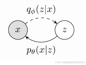
p
(
x
)
=
∫
z
p
θ
(
x
∣
z
)
p
(
z
)
p(x)=\int_z p_{\theta}(x|z)p(z)
p(x)=∫zpθ(x∣z)p(z)
p
(
x
)
=
∫
q
Φ
(
z
∣
x
)
p
θ
(
x
∣
z
)
p
(
z
)
q
Φ
(
z
∣
x
)
p(x)=\int q_{\Phi}(z|x)\frac{p_{\theta}(x|z)p(z)}{q_{\Phi}(z|x)}
p(x)=∫qΦ(z∣x)qΦ(z∣x)pθ(x∣z)p(z)
l
o
g
p
(
x
)
=
l
o
g
E
z
∼
q
ϕ
(
z
∣
x
)
[
p
θ
(
x
∣
z
)
p
(
z
)
q
ϕ
(
z
∣
x
)
]
log p(x)=log \mathbb{E}_{z\sim q_{\phi}(z|x)} [\frac{p_\theta(x|z)p(z)}{q_\phi(z|x)}]
logp(x)=logEz∼qϕ(z∣x)[qϕ(z∣x)pθ(x∣z)p(z)]
l
o
g
p
(
x
)
≥
l
o
g
E
z
∼
q
ϕ
(
z
∣
x
)
[
p
θ
(
x
∣
z
)
p
(
z
)
q
ϕ
(
z
∣
x
)
]
log p(x)\ge log \mathbb{E}_{z\sim q_{\phi}(z|x)} [\frac{p_\theta(x|z)p(z)}{q_\phi(z|x)}]
logp(x)≥logEz∼qϕ(z∣x)[qϕ(z∣x)pθ(x∣z)p(z)]
三、DDPM介绍
2020年Berkeley大学的学生提出的DDPM(Denoising Diffusion Probabilistic Models),简称扩散模型,是AIGC的核心算法,在生成图像的真实性和多样性方面均超越了GAN,而且训练过程稳定。
扩散模型包括两个过程:前向扩散过程(前向加噪过程)和反向去噪过程
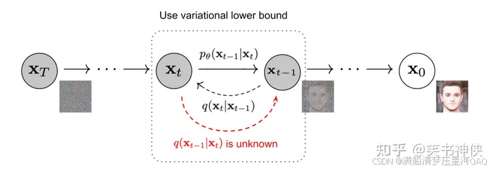
前向过程和反向过程都是马尔可夫链(有人可能对马尔科夫链比较陌生,这里打个不太恰当的比方,就好比明天的天气如何只以今天的天气作为变量和前天还有大前天都无关,也就是只和离他最近的一个结果有关,全过程大约需要1000步,其中反向过程用来生成数据,它的推导过程可以描述成:

四、前向扩散的过程
前向扩散过程是对原始数据逐渐增加高斯噪声,直至变成标准高斯分布的过程。
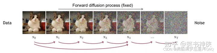
1)给定初始数据分布
x
0
∼
q
(
x
)
x_0 \sim q(x)
x0∼q(x),可以不断地向分布中添加高斯噪声,该噪声的标准差是以固定值
β
t
\beta_t
βt而确定的,均值是以固定值
β
t
\beta_{t}
βt和当前t-1时刻的数据
x
t
−
1
x_{t-1}
xt−1决定的,这个过程是一个马尔可夫过程。
2)随着t不断增大,最终数据分布 x T x_T xT变成了一个各项独立的高斯分布。
q ( x 1 : T ∣ x 0 ) = ∏ t = 1 T q ( x t ∣ x t − 1 ) q ( x t ∣ x t − 1 ) = N ( x t ; α t x t − 1 , β t I ) \begin{aligned} q(x_{1:T}|x_{0})&=\prod_{t=1}^{T}q(x_t|x_{t-1}) \\q(x_{t}|x_{t-1})&=\mathcal{N}(x_t;\sqrt{\alpha_t}x_{t-1},\beta_{t}I)\\ \end{aligned} q(x1:T∣x0)q(xt∣xt−1)=t=1∏Tq(xt∣xt−1)=N(xt;αtxt−1,βtI)
注: α t = 1 − β t \color{red}{\alpha_{t}=1-\beta_{t}} αt=1−βt!!!!这是作者设定
将 x t x_t xt 进行参数重整化,得到 x t = α t x t − 1 + β t ϵ t ϵ t ∼ N ( 0 , I ) \begin{aligned} x_{t}&=\sqrt{\alpha_{t}}x_{t-1}+\sqrt{\beta_{t}}\epsilon_{t} \space \space \space \space \epsilon_{t}\sim \mathcal{N}(0,I) \\ \end{aligned} xt=αtxt−1+βtϵt ϵt∼N(0,I)
3)任意时刻的 q ( x t ) q(x_t) q(xt) 推导也可以完全基于 x 0 x_0 x0和 β t \beta_t βt来计算出来,而不需要迭代
x t = α t x t − 1 + β t ϵ t = α t ( α t − 1 x t − 2 + β t − 1 ϵ t − 1 ) + β t ϵ t = α t α t − 1 ( α t − 2 x t − 3 + β t − 2 ϵ t − 2 ) + α t β t − 1 ϵ t − 1 + β t ϵ t = ( α t … α 1 ) x 0 + ( α t … α 2 ) β 1 ϵ 1 + ( α t … α 3 ) β 2 ϵ 2 + ⋯ + α t β t − 1 ϵ t − 1 + β t ϵ t \begin{aligned} x_{t}&=\sqrt{\alpha_{t}} x_{t-1}+\sqrt{\beta_{t}}\epsilon_{t}\\ &=\sqrt{\alpha_{t}}(\sqrt{\alpha_{t-1}}x_{t-2}+\sqrt{\beta_{t-1}}\epsilon_{t-1})+\sqrt{\beta_{t}}\epsilon_{t}\\ &=\sqrt{\alpha_{t}\alpha_{t-1}}(\sqrt{\alpha_{t-2}}x_{t-3}+\sqrt{\beta_{t-2}}\epsilon_{t-2})+\sqrt{\alpha_{t}\beta_{t-1}}\epsilon_{t-1}+\sqrt{\beta_{t}}\epsilon_{t}\\ &=\sqrt{(\alpha_{t}\dots\alpha_{1})}x_{0}+\sqrt{(\alpha_{t}\dots\alpha_{2})\beta_{1}}\epsilon_{1}+\sqrt{(\alpha_{t}\dots\alpha_{3})\beta_{2}}\epsilon_{2}+\dots+\sqrt{\alpha_{t}\beta_{t-1}}\epsilon_{t-1}+\sqrt{\beta_{t}}\epsilon_{t} \end{aligned} xt=αtxt−1+βtϵt=αt(αt−1xt−2+βt−1ϵt−1)+βtϵt=αtαt−1(αt−2xt−3+βt−2ϵt−2)+αtβt−1ϵt−1+βtϵt=(αt…α1)x0+(αt…α2)β1ϵ1+(αt…α3)β2ϵ2+⋯+αtβt−1ϵt−1+βtϵt
设: α t ˉ = α 1 α 2 … α t \bar{\alpha_{t}}=\alpha_{1}\alpha_{2}\dots\alpha_{t} αtˉ=α1α2…αt,接下来需要用到正态分布的叠加性
注意这里,两个正态分布
X
∼
N
(
μ
1
,
σ
1
)
X\sim N(\mu_1,\sigma_1)
X∼N(μ1,σ1)和
Y
∼
N
(
μ
2
,
σ
2
)
Y\sim N(\mu_2,\sigma_2)
Y∼N(μ2,σ2)的叠加后的分布
a
X
+
b
Y
aX+bY
aX+bY的均值为
a
μ
1
+
b
μ
2
a\mu_1+b\mu_2
aμ1+bμ2,方差为
a
2
σ
1
2
+
b
2
σ
2
2
a^2\sigma^2_1+b^2\sigma^2_2
a2σ12+b2σ22。所以
a
t
−
a
t
a
t
−
1
ϵ
t
−
2
+
1
−
a
t
ϵ
t
−
1
\sqrt{a_t-a_ta_{t-1}}\epsilon_{t-2}+\sqrt{1-a_t}\epsilon_{t-1}
at−atat−1ϵt−2+1−atϵt−1可以重参数化成只含一个随机变量
ϵ
\epsilon
ϵ构成的
1
−
a
t
a
t
−
1
ϵ
t
−
1
\sqrt{1-a_t a_{t-1}} \epsilon_{t-1}
1−atat−1ϵt−1
因此均值和方差可得:
μ
=
α
t
ˉ
σ
2
=
(
α
t
…
α
2
)
β
1
+
(
α
t
…
α
3
)
β
2
+
⋯
+
α
t
β
t
−
1
+
β
t
=
(
α
t
…
α
2
)
(
1
−
α
1
)
+
(
α
t
…
α
3
)
(
1
−
α
2
)
+
⋯
+
α
t
(
1
−
α
t
−
1
)
+
1
−
α
t
=
1
−
α
t
ˉ
\begin{aligned} \mu&=\sqrt{\bar{\alpha_{t}}}\\ \sigma^2&=(\alpha_{t}\dots\alpha_{2})\beta_{1}+(\alpha_{t}\dots\alpha_{3})\beta_{2}+\dots+\alpha_{t}\beta_{t-1}+\beta_{t}\\ &=(\alpha_{t}\dots\alpha_{2})(1-\alpha_{1})+(\alpha_{t}\dots\alpha_{3})(1-\alpha_{2})+\dots+\alpha_{t}(1-\alpha_{t-1})+1-\alpha_{t}\\ &=1-\bar{\alpha_{t}} \end{aligned}
μσ2=αtˉ=(αt…α2)β1+(αt…α3)β2+⋯+αtβt−1+βt=(αt…α2)(1−α1)+(αt…α3)(1−α2)+⋯+αt(1−αt−1)+1−αt=1−αtˉ
从而得到前向过程的最终表达式
x
t
=
α
t
ˉ
x
0
+
1
−
α
t
ˉ
ϵ
ϵ
∼
N
(
0
,
I
)
q
(
x
t
∣
x
0
)
=
N
(
x
t
;
α
t
ˉ
x
0
,
(
1
−
α
t
ˉ
)
I
)
\begin{aligned} x_{t}&=\sqrt{\bar{\alpha_{t}}}x_{0}+\sqrt{1-\bar{\alpha_{t}}}\epsilon \space \space\space \epsilon\sim \mathcal{N}(0,I)\\ q(x_{t}|x_{0})&=\mathcal{N}(x_{t};\sqrt{\bar{\alpha_{t}}}x_{0},(1-\bar{\alpha_{t}})I) \end{aligned}
xtq(xt∣x0)=αtˉx0+1−αtˉϵ ϵ∼N(0,I)=N(xt;αtˉx0,(1−αtˉ)I)
这个公式表示任意步骤t的噪声图像 x t x_t xt,都可以通过 x 0 x_0 x0直接加噪得到,后面需要用到。
五、反向去噪过程,神经网络拟合过程
反向去噪过程就是数据生成过程,它首先是从标准高斯分布中采样得到一个噪声样本,再一步步地迭代去噪,最后得到数据分布中的一个样本。
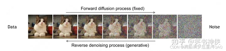
如果知道反向过程的每一步真实的条件分布
q
(
x
t
−
1
∣
x
t
)
q(x_{t-1}|x_t)
q(xt−1∣xt) ,那么从一个随机噪声开始,逐步采样就能生成一个真实的样本。但是真实的条件分布利用贝叶斯公式
q
(
x
t
−
1
∣
x
t
)
=
q
(
x
t
∣
x
t
−
1
)
q
(
x
t
−
1
)
q
(
x
t
)
q(x_{t-1}|x_{t}) =\frac{q(x_{t}|x_{t-1})q(x_{t-1})}{q(x_{t})}
q(xt−1∣xt)=q(xt)q(xt∣xt−1)q(xt−1)无法直接求解,原因是其中
q
(
x
t
−
1
)
,
q
(
x
t
)
q(x_{t-1}) ,q(x_{t})
q(xt−1),q(xt)未知,因此无法从
x
t
x_{t}
xt推导到
x
t
−
1
{x_{t-1}}
xt−1,所以必须通过神经网络
p
θ
(
x
t
−
1
∣
x
t
)
p_\theta(x_{t-1}|x_t)
pθ(xt−1∣xt) 来近似。为了简化起见,将反向过程也定义为一个马尔卡夫链,且服从高斯分布,建模如下:
p
θ
(
x
0
:
T
)
=
p
(
x
T
)
∏
t
=
1
T
p
θ
(
x
t
−
1
∣
x
t
)
p
θ
(
x
t
−
1
∣
x
t
)
=
N
(
x
t
−
1
;
μ
θ
(
x
t
,
t
)
,
∑
θ
(
x
t
,
t
)
)
p_\theta(x_{0:T})=p(x_T)\prod_{t=1}^Tp_\theta(x_{t-1}|x_t)\\ p_\theta(x_{t-1}|x_t)=N(x_{t-1};\mu_\theta(x_t,t),\sum_\theta(x_t,t))
pθ(x0:T)=p(xT)t=1∏Tpθ(xt−1∣xt)pθ(xt−1∣xt)=N(xt−1;μθ(xt,t),θ∑(xt,t))
虽然真实条件分布
q
(
x
t
−
1
∣
x
t
)
q(x_{t-1}|x_t)
q(xt−1∣xt)无法直接求解,但是加上已知条件
x
0
x_0
x0的后验分布
q
(
x
t
−
1
∣
x
t
,
x
0
)
q(x_{t-1}|x_{t},x_{0})
q(xt−1∣xt,x0)却可以通过贝叶斯公式求解,再结合前向马尔科夫性质可得:
q
(
x
t
−
1
∣
x
t
,
x
0
)
=
q
(
x
t
∣
x
t
−
1
,
x
0
)
q
(
x
t
−
1
∣
x
0
)
q
(
x
t
∣
x
0
)
=
q
(
x
t
∣
x
t
−
1
)
q
(
x
t
−
1
∣
x
0
)
q
(
x
t
∣
x
0
)
q(x_{t-1}|x_{t},x_{0}) =\frac{q(x_{t}|x_{t-1},x_{0})q(x_{t-1}|x_{0})}{q(x_{t}|x_{0})}=\frac{q(x_{t}|x_{t-1})q(x_{t-1}|x_{0})}{q(x_{t}|x_{0})}
q(xt−1∣xt,x0)=q(xt∣x0)q(xt∣xt−1,x0)q(xt−1∣x0)=q(xt∣x0)q(xt∣xt−1)q(xt−1∣x0)
因此可以得到:
q
(
x
t
−
1
∣
x
0
)
=
α
ˉ
t
−
1
x
0
+
1
−
α
ˉ
t
−
1
ϵ
∼
N
(
α
ˉ
t
−
1
x
0
,
(
1
−
α
ˉ
t
−
1
)
I
)
q
(
x
t
∣
x
0
)
=
α
ˉ
t
x
0
+
1
−
α
ˉ
t
ϵ
∼
N
(
α
ˉ
t
x
0
,
(
1
−
α
ˉ
t
)
I
)
q
(
x
t
∣
x
t
−
1
)
=
α
t
x
t
−
1
+
β
t
ϵ
∼
N
(
α
t
x
t
−
1
,
β
t
I
)
\begin{aligned} q(x_{t-1}|x_{0})&=\sqrt{\bar{\alpha}_{t-1}}x_{0}+\sqrt{1-\bar{\alpha}_{t-1}}\epsilon\sim \mathcal{N}(\sqrt{\bar{\alpha}_{t-1}}x_{0},(1-\bar{\alpha}_{t-1})I)\\ q(x_{t}|x_{0})&=\sqrt{\bar{\alpha}_{t}}x_{0}+\sqrt{1-\bar{\alpha}_{t}}\epsilon\sim \mathcal{N}(\sqrt{\bar{\alpha}_{t}}x_{0},(1-\bar{\alpha}_{t})I)\\ q(x_{t}|x_{t-1})&=\sqrt{\alpha}_{t}x_{t-1}+\beta_{t}\epsilon\sim \mathcal{N}(\sqrt{\alpha}_{t}x_{t-1},\beta_{t}I) \end{aligned}
q(xt−1∣x0)q(xt∣x0)q(xt∣xt−1)=αˉt−1x0+1−αˉt−1ϵ∼N(αˉt−1x0,(1−αˉt−1)I)=αˉtx0+1−αˉtϵ∼N(αˉtx0,(1−αˉt)I)=αtxt−1+βtϵ∼N(αtxt−1,βtI)
接下来需要用到:
所以
q
(
x
t
−
1
∣
x
t
,
x
0
)
∝
e
x
p
(
−
1
2
(
(
x
t
−
α
t
x
t
−
1
)
2
β
t
)
+
(
x
t
−
1
−
α
ˉ
t
−
1
x
0
)
2
1
−
α
ˉ
t
−
1
−
(
x
t
−
α
ˉ
t
x
0
)
2
1
−
α
ˉ
t
)
=
e
x
p
(
−
1
2
(
α
t
β
t
+
1
1
−
α
ˉ
t
−
1
)
x
t
−
1
2
−
(
2
α
t
β
t
x
t
+
2
α
t
ˉ
1
−
α
t
ˉ
x
0
)
x
t
−
1
+
C
(
x
t
,
x
0
)
)
\begin{aligned} q(x_{t-1}|x_{t},x_{0}) &\propto exp(-\frac{1}{2}(\frac{(x_{t}-\sqrt{\alpha_{t}}x_{t-1})^2}{\beta_{t}})+\frac{(x_{t-1}-\sqrt{\bar{\alpha}}_{t-1}x_{0})^2}{1-\bar{\alpha}_{t-1}}-\frac{(x_{t}-\sqrt{\bar{\alpha}_{t}}x_{0})^2}{1-\bar{\alpha}_{t}})\\ &=exp(-\frac{1}{2}(\color{red}{\frac{\alpha_{t}}{\beta_{t}}+\frac{1}{1-\bar{\alpha}_{t-1}}})x_{t-1}^2-(\color{blue}{\frac{2\sqrt{\alpha_{t}}}{\beta_{t}}x_{t}+\frac{2\sqrt{\bar{\alpha_{t}}}}{1-\bar{\alpha_{t}}}x_{0}})x_{t-1}+C(x_{t},x_{0})) \end{aligned}
q(xt−1∣xt,x0)∝exp(−21(βt(xt−αtxt−1)2)+1−αˉt−1(xt−1−αˉt−1x0)2−1−αˉt(xt−αˉtx0)2)=exp(−21(βtαt+1−αˉt−11)xt−12−(βt2αtxt+1−αtˉ2αtˉx0)xt−1+C(xt,x0))
通过配方就可以得到
β
~
t
=
1
/
(
α
t
β
t
+
1
1
−
α
ˉ
t
−
1
)
=
1
−
α
ˉ
t
−
1
1
−
α
ˉ
t
β
t
μ
~
t
=
(
α
t
β
t
x
t
+
α
ˉ
t
1
−
α
t
ˉ
x
0
)
/
(
α
t
β
t
+
1
1
−
α
ˉ
t
−
1
)
=
α
t
(
1
−
α
ˉ
t
−
1
)
1
−
α
t
ˉ
x
t
+
α
ˉ
t
−
1
β
t
1
−
α
ˉ
t
x
0
\widetilde{\beta}_t=1/(\frac{\alpha_{t}}{\beta_{t}}+\frac{1}{1-\bar{\alpha}_{t-1}})=\frac{1-\bar{\alpha}_{t-1}}{1-\bar{\alpha}_{t}}\beta_{t}\\ \widetilde{\mu}_t=(\frac{\sqrt\alpha_{t}}{\beta_{t}}x_{t}+\frac{\sqrt{\bar{\alpha}_{t}}}{1-\bar{\alpha_{t}}}x_{0})/(\frac{\alpha_{t}}{\beta_{t}}+\frac{1}{1-\bar{\alpha}_{t-1}})=\frac{\sqrt{\alpha_{t}}(1-\bar{\alpha}_{t-1})}{1-\bar{\alpha_{t}}}x_{t}+\frac{\sqrt{\bar{\alpha}_{t-1}}\beta_{t}}{1-\bar{\alpha}_{t}}x_{0}
β
t=1/(βtαt+1−αˉt−11)=1−αˉt1−αˉt−1βtμ
t=(βtαtxt+1−αtˉαˉtx0)/(βtαt+1−αˉt−11)=1−αtˉαt(1−αˉt−1)xt+1−αˉtαˉt−1βtx0
又因为由上面
x
0
x_0
x0和
x
t
x_t
xt的直接关系
x
0
=
1
α
ˉ
t
(
x
t
−
1
−
α
ˉ
t
ϵ
)
\color{red}{x_0= \frac{1}{\sqrt{\bar\alpha_t}}(x_t- {\sqrt{1-\bar \alpha_t} }\epsilon)}\\
x0=αˉt1(xt−1−αˉtϵ)
代入上式
μ
~
t
=
1
α
t
(
x
t
−
β
t
(
1
−
α
t
)
ϵ
)
\widetilde{\mu}_t=\frac{1}{\sqrt{\alpha_t} }(x_t-\frac{\beta_t}{\sqrt{(1-\alpha_t)}}\epsilon)
μ
t=αt1(xt−(1−αt)βtϵ)
这样我们就得到了后向过程
q
(
x
t
−
1
∣
x
t
,
x
0
)
q(x_{t-1}|x_t,x_0)
q(xt−1∣xt,x0)的均值和方差的公式,为了让
p
θ
(
x
t
−
1
∣
x
t
)
p_\theta(x_{t-1}|x_t)
pθ(xt−1∣xt)逼近
q
(
x
t
−
1
∣
x
t
,
x
0
)
q(x_{t-1}|x_t,x_0)
q(xt−1∣xt,x0)
我们固定住
∑
θ
(
x
t
,
t
)
=
β
t
\sum_\theta(x_t,t)=\beta_t
∑θ(xt,t)=βt和
∑
θ
(
x
t
,
t
)
=
β
~
t
\sum_\theta(x_t,t)=\widetilde{\beta}_t
∑θ(xt,t)=β
t,
β
t
\beta_t
βt和
β
~
t
\widetilde{\beta}_t
β
t其实大小是差不多的,但其实用
β
~
t
\widetilde{\beta}_t
β
t更好理解一点,因此只需要预测
μ
θ
(
x
t
,
t
)
\mu_{\theta}(x_t,t)
μθ(xt,t),又因为这里面只有
ϵ
\epsilon
ϵ是未知的,所以转而预测
ϵ
\epsilon
ϵ,因此均值可以写成下面的式子:
μ
θ
(
x
t
,
t
)
=
1
α
t
(
x
t
−
β
t
(
1
−
α
t
)
ϵ
θ
(
x
t
,
t
)
)
\mu_\theta(x_t,t)=\frac{1}{\sqrt{\alpha_t} }(x_t-\frac{\beta_t}{\sqrt{(1-\alpha_t)}}\epsilon_\theta(x_t,t))
μθ(xt,t)=αt1(xt−(1−αt)βtϵθ(xt,t))
注:
β
~
t
\widetilde\beta_t
β
t方差中没有未知参数
六、采样过程(模型训练完后的预测过程)
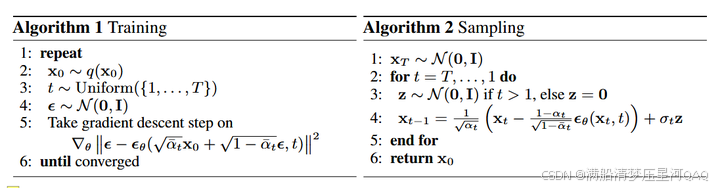
p θ ( x t − 1 ∣ x t ) = N ( x t − 1 ; μ θ ( x t , t ) , ∑ θ ( x t , t ) ) x t − 1 = 1 α t ( x t − β t ( 1 − α t ) ϵ θ ( x t , t ) ) + β ~ t z z ∼ N ( 0 , I ) p_\theta(x_{t-1}|x_t)=N(x_{t-1};\mu_\theta(x_t,t),\sum_\theta(x_t,t))\\ x_{t-1}=\frac{1}{\sqrt{\alpha_t} }(x_t-\frac{\beta_t}{\sqrt{(1-\alpha_t)}}\epsilon_\theta(x_t,t))+\sqrt{\widetilde{\beta}_t}z \space \space\space\space z\sim N(0,I) pθ(xt−1∣xt)=N(xt−1;μθ(xt,t),θ∑(xt,t))xt−1=αt1(xt−(1−αt)βtϵθ(xt,t))+β tz z∼N(0,I)
这里用z是为了和之前的 ϵ \epsilon ϵ区别开,都是符合正态分布的随机噪声,迭代1000次
七、优化目标
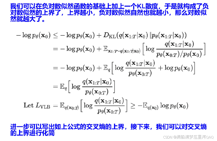
注意:
q
(
x
t
∣
x
t
−
1
)
=
q
(
x
t
∣
x
t
−
1
,
x
0
)
=
q
(
x
t
,
x
t
−
1
,
x
0
)
q
(
x
t
−
1
,
x
0
)
=
q
(
x
t
−
1
∣
x
t
,
x
0
)
q
(
x
t
∣
x
0
)
q
(
x
0
)
q
(
x
t
−
1
,
x
0
)
=
q
(
x
t
−
1
∣
x
t
,
x
0
)
q
(
x
t
∣
x
0
)
q
(
x
t
−
1
∣
x
0
)
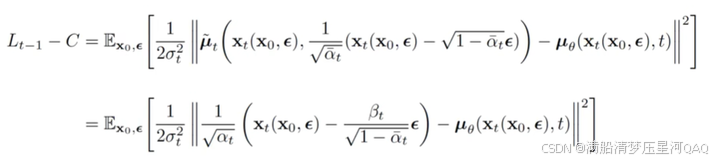
q(x_t|x_{t-1})=q(x_t|x_{t-1},x_0)=\frac{q(x_t,x_{t-1},x_0)}{q(x_{t-1},x_0)}=\frac{q(x_{t-1}|x_t,x_0)q(x_t|x_0)q(x_0)}{q(x_{t-1},x_0)}=\frac{q(x_{t-1}|x_t,x_0)q(x_t|x_0)}{q(x_{t-1}|x_0)}
q(xt∣xt−1)=q(xt∣xt−1,x0)=q(xt−1,x0)q(xt,xt−1,x0)=q(xt−1,x0)q(xt−1∣xt,x0)q(xt∣x0)q(x0)=q(xt−1∣x0)q(xt−1∣xt,x0)q(xt∣x0)
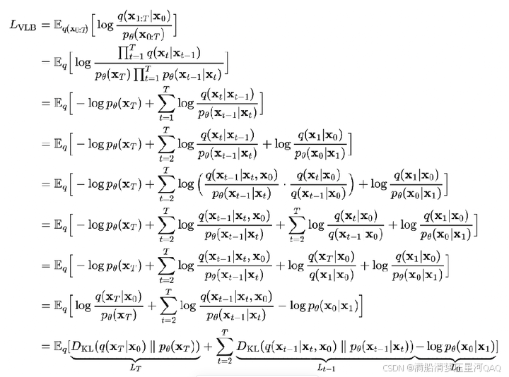
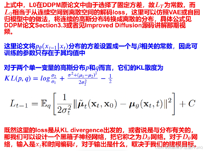

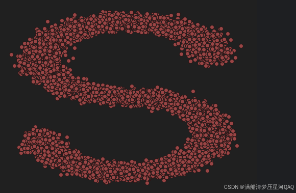
Code1:二维点demo
import torch
from matplotlib import pyplot as plt
import numpy as np
from sklearn.datasets import make_s_curve
from tqdm import tqdm

s_surve,_=make_s_curve(n_samples=10000,noise=0.1)
s_surve=s_surve[:,[0,2]]/10.0
print("shape of moons:",np.shape(s_surve))
data=s_surve.T
print(data.shape)
fig,ax=plt.subplots()
ax.scatter(*data,color="red",edgecolors="white")
ax.axis("off")
dataset = torch.Tensor(s_surve).float()
#制定每一步的beta
num_steps=100
betas=torch.linspace(-6,6,num_steps)
betas=torch.sigmoid(betas) *(0.5e-2-1e-5)+1e-5
#计算alpha、alpha_prod、alpha_prod_previous、alpha_bar_sqrt等变量的值
alphas=1-betas
alphas_prod=torch.cumprod(alphas,0)
alphas_prod_prev=torch.cat([torch.tensor([1]).float(),alphas_prod[:-1]],dim=0)
alphas_bar_sqrt=torch.sqrt(alphas_prod)
one_minus_alphas_bar_log=torch.log(1-alphas_prod)
one_minus_alphas_bar_sqrt=torch.sqrt(1-alphas_prod)
assert alphas.shape==alphas_prod.shape==alphas_prod_prev.shape==alphas_bar_sqrt.shape==one_minus_alphas_bar_log.shape==one_minus_alphas_bar_sqrt.shape
print(alphas.shape)

def q_x(x_0,t):
    noise=torch.randn_like(x_0)
    alphas_t=alphas_bar_sqrt[t]
    alphas_1_m_t=one_minus_alphas_bar_sqrt[t]
    return (alphas_t*x_0+alphas_1_m_t*noise)

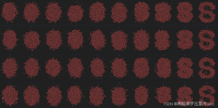
num_shows=20
fig,axs=plt.subplots(2,10,figsize=(28,3))
plt.rc("text",color="blue")
#共有10000个点,每个店包含两个坐标
#生成100步以内每隔5步加噪声后的图像

for i in range(num_shows):
    j=i//10
    k=i%10
    q_i=q_x(dataset,torch.tensor([i*num_steps//num_shows]))
    axs[j,k].scatter(q_i[:,0],q_i[:,1],color="red",edgecolors="white")
    axs[j,k].axis("off")
    axs[j,k].set_title(str(i))
import torch
import torch.nn as nn

class MLPDiffusion(nn.Module):
    def __init__(self,n_steps,num_units=128):
        super().__init__()
        self.linears=nn.ModuleList(
            [
            nn.Linear(2,num_units),
            nn.ReLU(),
            nn.Linear(num_units,num_units),
            nn.ReLU(),
            nn.Linear(num_units,num_units),
            nn.ReLU(),
            nn.Linear(num_units,2)
            ]

        )
        self.step_embeddings=nn.ModuleList(
            [
                nn.Embedding(n_steps,num_units),
                nn.Embedding(n_steps,num_units),
                nn.Embedding(n_steps,num_units),
            ]
        )
    def forward(self,x,t):
        for idx,embedding_layer in enumerate(self.step_embeddings):
            t_embedding=embedding_layer(t)
            x=self.linears[2*idx](x)
            x+=t_embedding
            x=self.linears[2*idx+1](x)
        x=self.linears[-1](x)
        return x

def diffusion_loss_fn(model,x_0,alphas_bar_sqrt,one_minus_alphas_bar_sqrt,n_steps):
    batch_size=x_0.shape[0]
    #对一个batchsize样本生成随机时刻t
    t=torch.randint(0,n_steps,size=(batch_size//2,))
    t=torch.cat([t,n_steps-1-t],dim=0)
    t=t.unsqueeze(-1)
    #x0系数
    a=alphas_bar_sqrt[t]
    #eps的系数
    aml=one_minus_alphas_bar_sqrt[t]
    #生成随机噪音eps
    e=torch.randn_like(x_0)

    #构造模型的输入
    x=x_0*a+e*aml

    #送入模型,得到t时刻的随机噪声预测值
    output=model(x,t.squeeze(-1))

    #与真实噪声一起计算误差,求平均值
    return (e-output).square().mean()

def p_sample_loop(model,shape,n_steps,betas,one_minus_alphas_bar_sqrt):
    cur_x=torch.randn(shape)
    x_seq=[cur_x]
    for i in reversed(range(n_steps)):
        cur_x=p_sample(model,cur_x,i,betas,one_minus_alphas_bar_sqrt)
        x_seq.append(cur_x)
    return x_seq

def p_sample(model,x,t,betas,one_minus_alphas_bar_sqrt):
    #从x[T]采样t时刻的重构值
    t=torch.tensor([t])
    coeff=betas[t]/one_minus_alphas_bar_sqrt[t]
    eps_theta=model(x,t)
    mean=(1/(1-betas[t]).sqrt())*(x-(coeff*eps_theta))
    z=torch.randn_like(x)
    sigma_t=betas[t].sqrt()
    sample=mean+sigma_t*z
    return sample

seed=1234
class EMA:
    def __init__(self,mu=0.0):
        self.mu=mu
        self.shadow={}
    def register(self,name,val):
        self.shadow[name]=val.clone()

    def __call__(self,name,x):
        assert name in self.shadow
        new_average=self.mu*x+(1.0-self.mu)*self.shadow[name]
        self.shadow[name]=new_average.clone()
        return new_average

print("Training model")

batch_size=128
dataloader=torch.utils.data.DataLoader(dataset, batch_size,shuffle=True)
num_epoch=4000
plt.rc("text",color="blue")
model=MLPDiffusion(num_steps)
optimzer=torch.optim.Adam(model.parameters(),lr=1e-3)

for t in range(num_epoch):
    for idx,batch_x in enumerate(dataloader):
        loss=diffusion_loss_fn(model,batch_x,alphas_bar_sqrt,one_minus_alphas_bar_sqrt,num_steps)
        optimzer.zero_grad()
        loss.backward()
        torch.nn.utils.clip_grad_norm_(model.parameters(),1.0)
        optimzer.step()
    if(t%100==0):
        print(loss)
        x_seq=p_sample_loop(model,dataset.shape,num_steps,betas,one_minus_alphas_bar_sqrt)
        fig,axs=plt.subplots(1,10,figsize=(28,3))
        for i in range(1,11):
            cur_x=x_seq[i*10].detach()
            axs[i-1].scatter(cur_x[:,0],cur_x[:,1],color="red",edgecolors="white")
            axs[i-1].axis("off")
            axs[i-1].set_title(str(i))
import io
from PIL import Image
imgs=[]
for i in range(100):
    plt.clf()
    q_i=q_x(dataset,torch.tensor([i]))
    plt.scatter(q_i[:,0],q_i[:,1],color="red",edgecolors="white",s=5)
    plt.axis("off")

    img_buf=io.BytesIO()
    plt.savefig(img_buf,format="png")
    img=Image.open(img_buf)
    imgs.append(img)
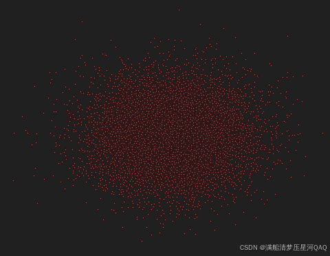
reverse=[]
for i in range(100):
    plt.clf()
    cur_x=x_seq[i].detach()
    plt.scatter(cur_x[:,0],cur_x[:,1],color="red",edgecolors="white",s=5)
    plt.axis("off")

    img_buf=io.BytesIO()
    plt.savefig(img_buf,format="png")
    img=Image.open(img_buf)
    imgs.append(img)
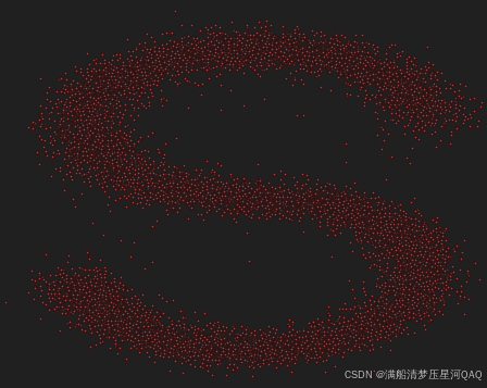
Code2:图片Demo
import torch
import torchvision
import matplotlib.pyplot as plt
import torch.nn.functional as F
from torchvision import transforms
from torch.utils.data import DataLoader
import numpy as np
from torch.optim import Adam
from torch import nn
import math
from torchvision.utils import save_image


def show_images(data, num_samples=20, cols=4):
    """ Plots some samples from the dataset """
    plt.figure(figsize=(15,15))
    for i, img in enumerate(data):
        if i == num_samples:
            break
        plt.subplot(int(num_samples/cols) + 1, cols, i + 1)
        plt.imshow(img[0])


def linear_beta_schedule(timesteps, start=0.0001, end=0.02):
    return torch.linspace(start, end, timesteps)


def get_index_from_list(vals, t, x_shape):
    """
    Returns a specific index t of a passed list of values vals
    while considering the batch dimension.
    """
    batch_size = t.shape[0]
    out = vals.gather(-1, t.cpu())
    #print("out:",out)
    #print("out.shape:",out.shape)
    return out.reshape(batch_size, *((1,) * (len(x_shape) - 1))).to(t.device)

def forward_diffusion_sample(x_0, t, device="cpu"):
    """
    Takes an image and a timestep as input and
    returns the noisy version of it
    """
    noise = torch.randn_like(x_0)
    sqrt_alphas_cumprod_t = get_index_from_list(sqrt_alphas_cumprod, t, x_0.shape)
    sqrt_one_minus_alphas_cumprod_t = get_index_from_list(
        sqrt_one_minus_alphas_cumprod, t, x_0.shape
    )
    # mean + variance
    return sqrt_alphas_cumprod_t.to(device) * x_0.to(device) \
    + sqrt_one_minus_alphas_cumprod_t.to(device) * noise.to(device), noise.to(device)


def load_transformed_dataset(IMG_SIZE):
    data_transforms = [
        transforms.Resize((IMG_SIZE, IMG_SIZE)),
        transforms.ToTensor(), # Scales data into [0,1]
        transforms.Lambda(lambda t: (t * 2) - 1) # Scale between [-1, 1]
    ]
    data_transform = transforms.Compose(data_transforms)

    train = torchvision.datasets.MNIST(root="./Data",transform=data_transform,train=True)
    test = torchvision.datasets.MNIST(root="./Data", transform=data_transform, train=False)

    return torch.utils.data.ConcatDataset([train, test])

def show_tensor_image(image):
    reverse_transforms = transforms.Compose([
        transforms.Lambda(lambda t: (t + 1) / 2),
        transforms.Lambda(lambda t: t.permute(1, 2, 0)), # CHW to HWC
        transforms.Lambda(lambda t: t * 255.),
        transforms.Lambda(lambda t: t.numpy().astype(np.uint8)),
        transforms.ToPILImage(),
    ])

    #Take first image of batch
    if len(image.shape) == 4:
        image = image[0, :, :, :]
    plt.imshow(reverse_transforms(image))


class Block(nn.Module):
    def __init__(self, in_ch, out_ch, time_emb_dim, up=False):
        super().__init__()
        self.time_mlp =  nn.Linear(time_emb_dim, out_ch)
        if up:
            self.conv1 = nn.Conv2d(2*in_ch, out_ch, 3, padding=1)
            self.transform = nn.ConvTranspose2d(out_ch, out_ch, 4, 2, 1)
        else:
            self.conv1 = nn.Conv2d(in_ch, out_ch, 3, padding=1)
            self.transform = nn.Conv2d(out_ch, out_ch, 4, 2, 1)
        self.conv2 = nn.Conv2d(out_ch, out_ch, 3, padding=1)
        self.bnorm1 = nn.BatchNorm2d(out_ch)
        self.bnorm2 = nn.BatchNorm2d(out_ch)
        self.relu  = nn.ReLU()

    def forward(self, x, t):
        #print("ttt:",t.shape)
        # First Conv
        h = self.bnorm1(self.relu(self.conv1(x)))
        # Time embedding
        time_emb = self.relu(self.time_mlp(t))
        # Extend last 2 dimensions
        time_emb = time_emb[(..., ) + (None, ) * 2]
        # Add time channel
        h = h + time_emb
        # Second Conv
        h = self.bnorm2(self.relu(self.conv2(h)))
        # Down or Upsample
        return self.transform(h)


class SinusoidalPositionEmbeddings(nn.Module):
    def __init__(self, dim):
        super().__init__()
        self.dim = dim

    def forward(self, time):
        device = time.device
        half_dim = self.dim // 2
        embeddings = math.log(10000) / (half_dim - 1)
        embeddings = torch.exp(torch.arange(half_dim, device=device) * -embeddings)
        embeddings = time[:, None] * embeddings[None, :]
        embeddings = torch.cat((embeddings.sin(), embeddings.cos()), dim=-1)
        # TODO: Double check the ordering here
        return embeddings


class SimpleUnet(nn.Module):
    """
    A simplified variant of the Unet architecture.
    """
    def __init__(self):
        super().__init__()
        image_channels =1   #灰度图为1,彩色图为3
        down_channels = (64, 128, 256, 512, 1024)
        up_channels = (1024, 512, 256, 128, 64)
        out_dim = 1   #灰度图为1 ,彩色图为3
        time_emb_dim = 32

        # Time embedding
        self.time_mlp = nn.Sequential(
                SinusoidalPositionEmbeddings(time_emb_dim),
                nn.Linear(time_emb_dim, time_emb_dim),
                nn.ReLU()
            )

        # Initial projection
        self.conv0 = nn.Conv2d(image_channels, down_channels[0], 3, padding=1)

        # Downsample
        self.downs = nn.ModuleList([Block(down_channels[i], down_channels[i+1], \
                                    time_emb_dim) \
                    for i in range(len(down_channels)-1)])
        # Upsample
        self.ups = nn.ModuleList([Block(up_channels[i], up_channels[i+1], \
                                        time_emb_dim, up=True) \
                    for i in range(len(up_channels)-1)])

        # Edit: Corrected a bug found by Jakub C (see YouTube comment)
        self.output = nn.Conv2d(up_channels[-1], out_dim, 1)

    def forward(self, x, timestep):
        # Embedd time
        t = self.time_mlp(timestep)
        # Initial conv
        x = self.conv0(x)
        # Unet
        residual_inputs = []
        for down in self.downs:
            x = down(x, t)
            residual_inputs.append(x)
        for up in self.ups:
            residual_x = residual_inputs.pop()
            # Add residual x as additional channels
            x = torch.cat((x, residual_x), dim=1)
            x = up(x, t)
        return self.output(x)


def get_loss(model, x_0, t):
    x_noisy, noise = forward_diffusion_sample(x_0, t, device)
    noise_pred = model(x_noisy, t)
    return F.l1_loss(noise, noise_pred)


@torch.no_grad()
def sample_timestep(x, t):
    """
    Calls the model to predict the noise in the image and returns
    the denoised image.
    Applies noise to this image, if we are not in the last step yet.
    """
    betas_t = get_index_from_list(betas, t, x.shape)
    sqrt_one_minus_alphas_cumprod_t = get_index_from_list(
        sqrt_one_minus_alphas_cumprod, t, x.shape
    )

    sqrt_recip_alphas_t = get_index_from_list(sqrt_recip_alphas, t, x.shape)

    # Call model (current image - noise prediction)
    model_mean = sqrt_recip_alphas_t * (
        x - betas_t * model(x, t) / sqrt_one_minus_alphas_cumprod_t
    )

    posterior_variance_t = get_index_from_list(posterior_variance, t, x.shape)

    if t == 0:
        # As pointed out by Luis Pereira (see YouTube comment)
        # The t's are offset from the t's in the paper
        return model_mean
    else:
        noise = torch.randn_like(x)
        return model_mean + torch.sqrt(posterior_variance_t) * noise

@torch.no_grad()
def sample_plot_image(IMG_SIZE):
    # Sample noise
    img_size = IMG_SIZE
    img = torch.randn((1, 1, img_size, img_size), device=device)   #生成第T步的图片
    plt.figure(figsize=(15,15))
    plt.axis('off')
    num_images = 10
    stepsize = int(T/num_images)

    for i in range(0,T)[::-1]:
        t = torch.full((1,), i, device=device, dtype=torch.long)
        #print("t:",t)
        img = sample_timestep(img, t)
        # Edit: This is to maintain the natural range of the distribution
        img = torch.clamp(img, -1.0, 1.0)
        if i % stepsize == 0:
            plt.subplot(1, num_images, int(i/stepsize)+1)
            plt.title(str(i))
            show_tensor_image(img.detach().cpu())
    plt.show()


if __name__ =="__main__":

    # Define beta schedule
    T = 300
    betas = linear_beta_schedule(timesteps=T)

    # Pre-calculate different terms for closed form
    alphas = 1. - betas
    alphas_cumprod = torch.cumprod(alphas, axis=0)
    # print(alphas_cumprod.shape)
    alphas_cumprod_prev = F.pad(alphas_cumprod[:-1], (1, 0), value=1.0)
    # print(alphas_cumprod_prev)
    # print(alphas_cumprod_prev.shape)
    sqrt_recip_alphas = torch.sqrt(1.0 / alphas)
    sqrt_alphas_cumprod = torch.sqrt(alphas_cumprod)
    sqrt_one_minus_alphas_cumprod = torch.sqrt(1. - alphas_cumprod)
    posterior_variance = betas * (1. - alphas_cumprod_prev) / (1. - alphas_cumprod)
    # print(posterior_variance.shape)


    IMG_SIZE = 32
    BATCH_SIZE = 16

    data = load_transformed_dataset(IMG_SIZE)
    dataloader = DataLoader(data, batch_size=BATCH_SIZE, shuffle=True, drop_last=True)

    model = SimpleUnet()
    print("Num params: ", sum(p.numel() for p in model.parameters()))

    device = "cuda" if torch.cuda.is_available() else "cpu"
    model.to(device)
    optimizer = Adam(model.parameters(), lr=0.001)
    epochs = 1 # Try more!

    for epoch in range(epochs):
        for step, batch in enumerate(dataloader):  #由于batch 是包含标签的所以取batch[0]
            #print(batch[0].shape)
            optimizer.zero_grad()

            t = torch.randint(0, T, (BATCH_SIZE,), device=device).long()
            loss = get_loss(model, batch[0], t)
            loss.backward()
            optimizer.step()

            if epoch % 1 == 0 and step %5== 0:
                print(f"Epoch {epoch} | step {step:03d} Loss: {loss.item()} ")
                sample_plot_image(IMG_SIZE)
参考文献
https://zhuanlan.zhihu.com/p/630354327
https://blog.csdn.net/weixin_45453121/article/details/131223653
https://www.cnblogs.com/risejl/p/17448442.html
https://zhuanlan.zhihu.com/p/569994589?utm_id=0
更多推荐

 9
9 0
0- 0


 已为社区贡献4条内容

所有评论(0)