
机器学习与深度学习day9——热力图与子图绘制
本节课主要学习:
1. 相关系数热力图的绘制与解读
2. 子图布局的创建与使用
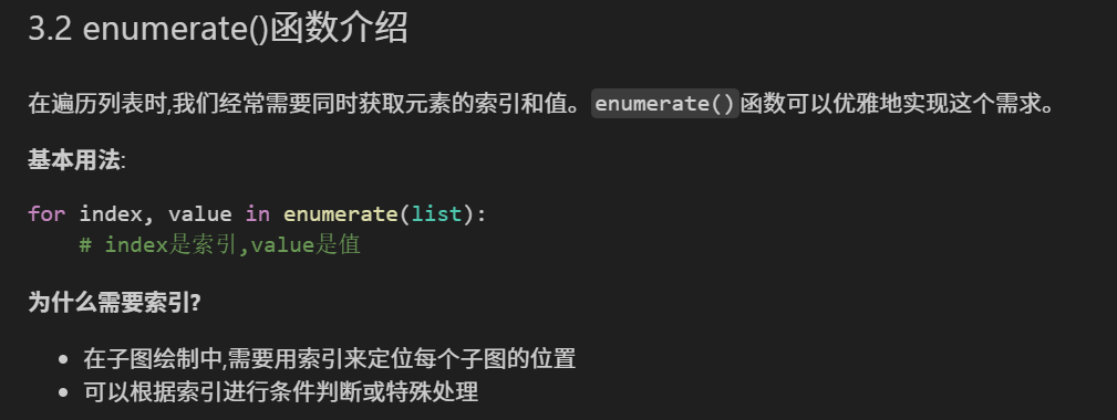
3. enumerate()函数的实用技巧
学习目标: 掌握多变量关系的可视化方法,学会使用子图进行批量绘图。
一、数据预处理回顾
在进行可视化分析之前,我们需要先完成数据的基本清洗和转换工作。
# 首先走一遍完整的之前的流程
# 读取数据
import warnings
warnings.filterwarnings('ignore')
import pandas as pd
data  = pd.read_csv('data.csv')
# 查看数据
data.info()
<class 'pandas.core.frame.DataFrame'>
RangeIndex: 7500 entries, 0 to 7499
Data columns (total 18 columns):
# Column Non-Null Count Dtype
--- ------ -------------- -----
0 Id 7500 non-null int64
1 Home Ownership 7500 non-null object
2 Annual Income 5943 non-null float64
3 Years in current job 7129 non-null object
4 Tax Liens 7500 non-null float64
5 Number of Open Accounts 7500 non-null float64
6 Years of Credit History 7500 non-null float64
7 Maximum Open Credit 7500 non-null float64
8 Number of Credit Problems 7500 non-null float64
9 Months since last delinquent 3419 non-null float64
10 Bankruptcies 7486 non-null float64
11 Purpose 7500 non-null object
12 Term 7500 non-null object
13 Current Loan Amount 7500 non-null float64
14 Current Credit Balance 7500 non-null float64
15 Monthly Debt 7500 non-null float64
16 Credit Score 5943 non-null float64
17 Credit Default 7500 non-null int64
dtypes: float64(12), int64(2), object(4)
memory usage: 1.0+ MB
data.head()
| Id | Home Ownership | Annual Income | Years in current job | Tax Liens | Number of Open Accounts | Years of Credit History | Maximum Open Credit | Number of Credit Problems | Months since last delinquent | Bankruptcies | Purpose | Term | Current Loan Amount | Current Credit Balance | Monthly Debt | Credit Score | Credit Default | |
|---|---|---|---|---|---|---|---|---|---|---|---|---|---|---|---|---|---|---|
| 0 | 0 | Own Home | 482087.0 | NaN | 0.0 | 11.0 | 26.3 | 685960.0 | 1.0 | NaN | 1.0 | debt consolidation | Short Term | 99999999.0 | 47386.0 | 7914.0 | 749.0 | 0 |
| 1 | 1 | Own Home | 1025487.0 | 10+ years | 0.0 | 15.0 | 15.3 | 1181730.0 | 0.0 | NaN | 0.0 | debt consolidation | Long Term | 264968.0 | 394972.0 | 18373.0 | 737.0 | 1 |
| 2 | 2 | Home Mortgage | 751412.0 | 8 years | 0.0 | 11.0 | 35.0 | 1182434.0 | 0.0 | NaN | 0.0 | debt consolidation | Short Term | 99999999.0 | 308389.0 | 13651.0 | 742.0 | 0 |
| 3 | 3 | Own Home | 805068.0 | 6 years | 0.0 | 8.0 | 22.5 | 147400.0 | 1.0 | NaN | 1.0 | debt consolidation | Short Term | 121396.0 | 95855.0 | 11338.0 | 694.0 | 0 |
| 4 | 4 | Rent | 776264.0 | 8 years | 0.0 | 13.0 | 13.6 | 385836.0 | 1.0 | NaN | 0.0 | debt consolidation | Short Term | 125840.0 | 93309.0 | 7180.0 | 719.0 | 0 |
1.1 特征映射准备
对于包含字符串的分类特征,需要先转换为数值型才能进行后续的相关性分析。
# 把years in current job列和Home Ownership列转化为数字
# 先查看内容
data["Years in current job"].value_counts()
Years in current job
10+ years 2332
2 years 705
3 years 620
< 1 year 563
5 years 516
1 year 504
4 years 469
6 years 426
7 years 396
8 years 339
9 years 259
Name: count, dtype: int64
data["Home Ownership"].value_counts()
Home Ownership
Home Mortgage 3637
Rent 3204
Own Home 647
Have Mortgage 12
Name: count, dtype: int64
1.2 使用嵌套字典进行特征映射
为什么使用嵌套字典?
- 集中管理多个特征的映射规则
- 代码结构清晰,易于维护
- 方便批量处理多个特征
# 创建嵌套字典用于映射
mappings = {
    "Years in current job": {
        "10+ years": 10,
        "2 years": 2,
        "3 years": 3,
        "< 1 year": 0,
        "5 years": 5,
        "1 year": 1,
        "4 years": 4,
        "6 years": 6,
        "7 years": 7,
        "8 years": 8,
        "9 years": 9
    },
    "Home Ownership": {
        "Home Mortgage": 0,
        "Rent": 1,
        "Own Home": 2,
        "Have Mortgage": 3
    }
}
# 使用映射字典进行转换
data["Years in current job"] = data["Years in current job"].map(mappings["Years in current job"])
data["Home Ownership"] = data["Home Ownership"].map(mappings["Home Ownership"])
data.info()
<class 'pandas.core.frame.DataFrame'>
RangeIndex: 7500 entries, 0 to 7499
Data columns (total 18 columns):
# Column Non-Null Count Dtype
--- ------ -------------- -----
0 Id 7500 non-null int64
1 Home Ownership 7500 non-null int64
2 Annual Income 5943 non-null float64
3 Years in current job 7129 non-null float64
4 Tax Liens 7500 non-null float64
5 Number of Open Accounts 7500 non-null float64
6 Years of Credit History 7500 non-null float64
7 Maximum Open Credit 7500 non-null float64
8 Number of Credit Problems 7500 non-null float64
9 Months since last delinquent 3419 non-null float64
10 Bankruptcies 7486 non-null float64
11 Purpose 7500 non-null object
12 Term 7500 non-null object
13 Current Loan Amount 7500 non-null float64
14 Current Credit Balance 7500 non-null float64
15 Monthly Debt 7500 non-null float64
16 Credit Score 5943 non-null float64
17 Credit Default 7500 non-null int64
dtypes: float64(13), int64(3), object(2)
memory usage: 1.0+ MB
data.head()
| Id | Home Ownership | Annual Income | Years in current job | Tax Liens | Number of Open Accounts | Years of Credit History | Maximum Open Credit | Number of Credit Problems | Months since last delinquent | Bankruptcies | Purpose | Term | Current Loan Amount | Current Credit Balance | Monthly Debt | Credit Score | Credit Default | |
|---|---|---|---|---|---|---|---|---|---|---|---|---|---|---|---|---|---|---|
| 0 | 0 | 2 | 482087.0 | NaN | 0.0 | 11.0 | 26.3 | 685960.0 | 1.0 | NaN | 1.0 | debt consolidation | Short Term | 99999999.0 | 47386.0 | 7914.0 | 749.0 | 0 |
| 1 | 1 | 2 | 1025487.0 | 10.0 | 0.0 | 15.0 | 15.3 | 1181730.0 | 0.0 | NaN | 0.0 | debt consolidation | Long Term | 264968.0 | 394972.0 | 18373.0 | 737.0 | 1 |
| 2 | 2 | 0 | 751412.0 | 8.0 | 0.0 | 11.0 | 35.0 | 1182434.0 | 0.0 | NaN | 0.0 | debt consolidation | Short Term | 99999999.0 | 308389.0 | 13651.0 | 742.0 | 0 |
| 3 | 3 | 2 | 805068.0 | 6.0 | 0.0 | 8.0 | 22.5 | 147400.0 | 1.0 | NaN | 1.0 | debt consolidation | Short Term | 121396.0 | 95855.0 | 11338.0 | 694.0 | 0 |
| 4 | 4 | 1 | 776264.0 | 8.0 | 0.0 | 13.0 | 13.6 | 385836.0 | 1.0 | NaN | 0.0 | debt consolidation | Short Term | 125840.0 | 93309.0 | 7180.0 | 719.0 | 0 |
1.3 特征名中文映射
为了更好地理解数据,我们将英文特征名映射为中文特征名。
为什么需要中文映射?
- 提高可读性,更容易理解特征含义
- 方便团队沟通和报告展示
- 在热力图等可视化中展示更友好
data.columns
Index(['Id', 'Home Ownership', 'Annual Income', 'Years in current job',
'Tax Liens', 'Number of Open Accounts', 'Years of Credit History',
'Maximum Open Credit', 'Number of Credit Problems',
'Months since last delinquent', 'Bankruptcies', 'Purpose', 'Term',
'Current Loan Amount', 'Current Credit Balance', 'Monthly Debt',
'Credit Score', 'Credit Default'],
dtype='object')
# 创建特征名中文映射字典
feature_name_mapping = {
    'Annual Income': '年收入',
    'Years in current job': '当前工作年限',
    'Tax Liens': '税收留置权',
    'Number of Open Accounts': '开放账户数量',
    'Years of Credit History': '信用历史年限',
    'Maximum Open Credit': '最大开放信用额度',
    'Number of Credit Problems': '信用问题数量',
    'Months since last delinquent': '距上次拖欠月数',
    'Bankruptcies': '破产次数',
    'Current Loan Amount': '当前贷款金额',
    'Current Credit Balance': '当前信用余额',
    'Monthly Debt': '月债务',
    'Credit Score': '信用评分',
    'Home Ownership': '房屋所有权',
    'Term': '贷款期限',
    'Purpose': '贷款目的',
    'Credit Default': '信用违约'
}

# 重命名数据框的列名
data_cn = data.rename(columns=feature_name_mapping)
data_cn.head()
| Id | 房屋所有权 | 年收入 | 当前工作年限 | 税收留置权 | 开放账户数量 | 信用历史年限 | 最大开放信用额度 | 信用问题数量 | 距上次拖欠月数 | 破产次数 | 贷款目的 | 贷款期限 | 当前贷款金额 | 当前信用余额 | 月债务 | 信用评分 | 信用违约 | |
|---|---|---|---|---|---|---|---|---|---|---|---|---|---|---|---|---|---|---|
| 0 | 0 | 2 | 482087.0 | NaN | 0.0 | 11.0 | 26.3 | 685960.0 | 1.0 | NaN | 1.0 | debt consolidation | Short Term | 99999999.0 | 47386.0 | 7914.0 | 749.0 | 0 |
| 1 | 1 | 2 | 1025487.0 | 10.0 | 0.0 | 15.0 | 15.3 | 1181730.0 | 0.0 | NaN | 0.0 | debt consolidation | Long Term | 264968.0 | 394972.0 | 18373.0 | 737.0 | 1 |
| 2 | 2 | 0 | 751412.0 | 8.0 | 0.0 | 11.0 | 35.0 | 1182434.0 | 0.0 | NaN | 0.0 | debt consolidation | Short Term | 99999999.0 | 308389.0 | 13651.0 | 742.0 | 0 |
| 3 | 3 | 2 | 805068.0 | 6.0 | 0.0 | 8.0 | 22.5 | 147400.0 | 1.0 | NaN | 1.0 | debt consolidation | Short Term | 121396.0 | 95855.0 | 11338.0 | 694.0 | 0 |
| 4 | 4 | 1 | 776264.0 | 8.0 | 0.0 | 13.0 | 13.6 | 385836.0 | 1.0 | NaN | 0.0 | debt consolidation | Short Term | 125840.0 | 93309.0 | 7180.0 | 719.0 | 0 |
二、相关系数热力图
2.1 什么是相关系数热力图?
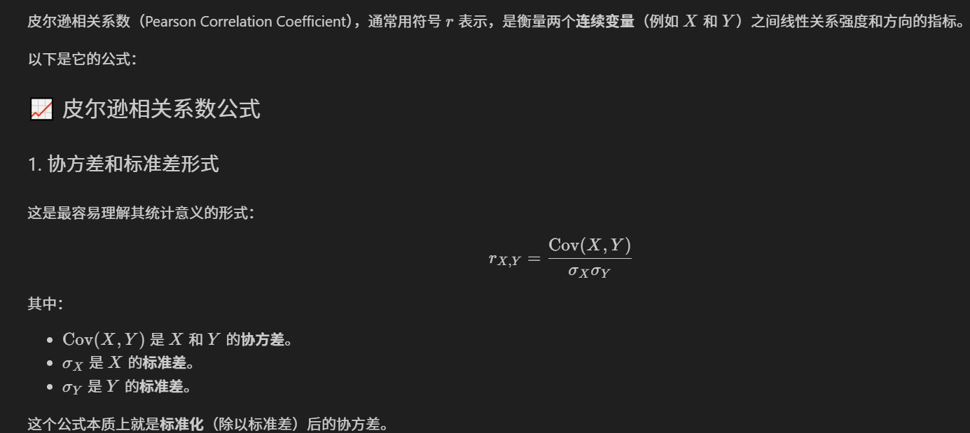
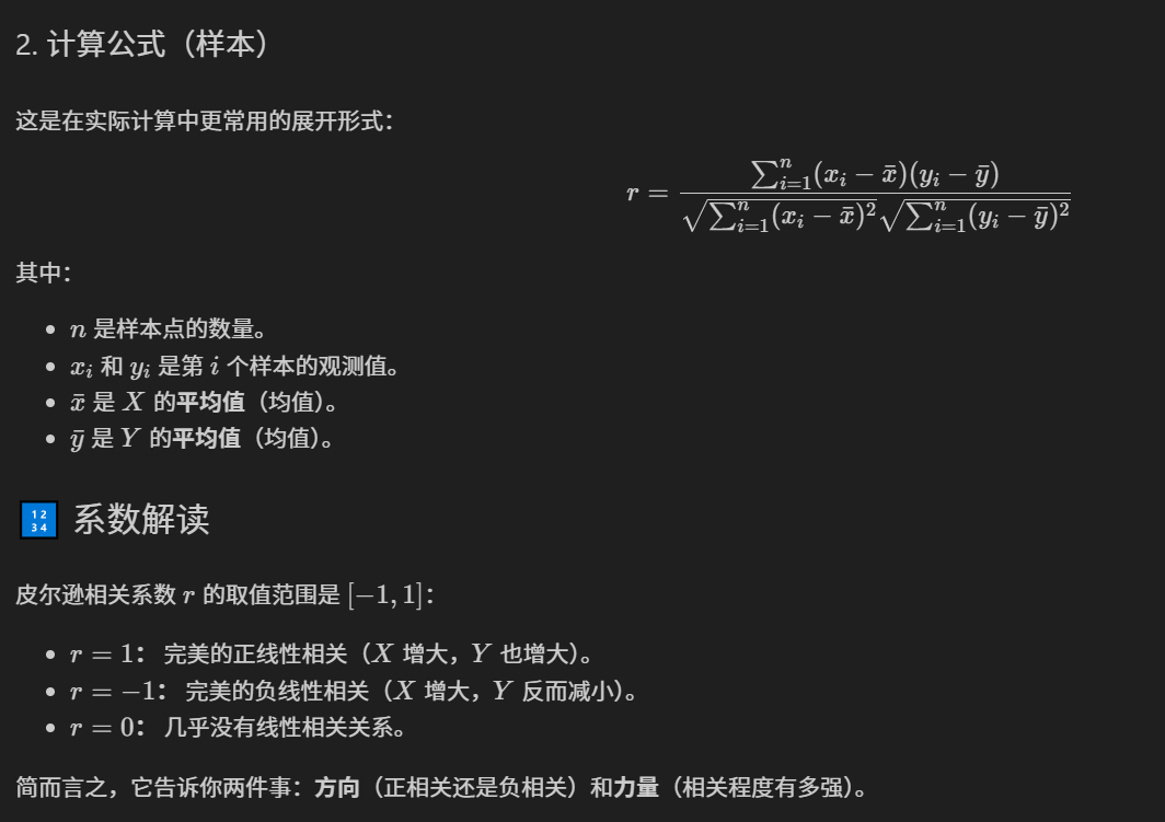
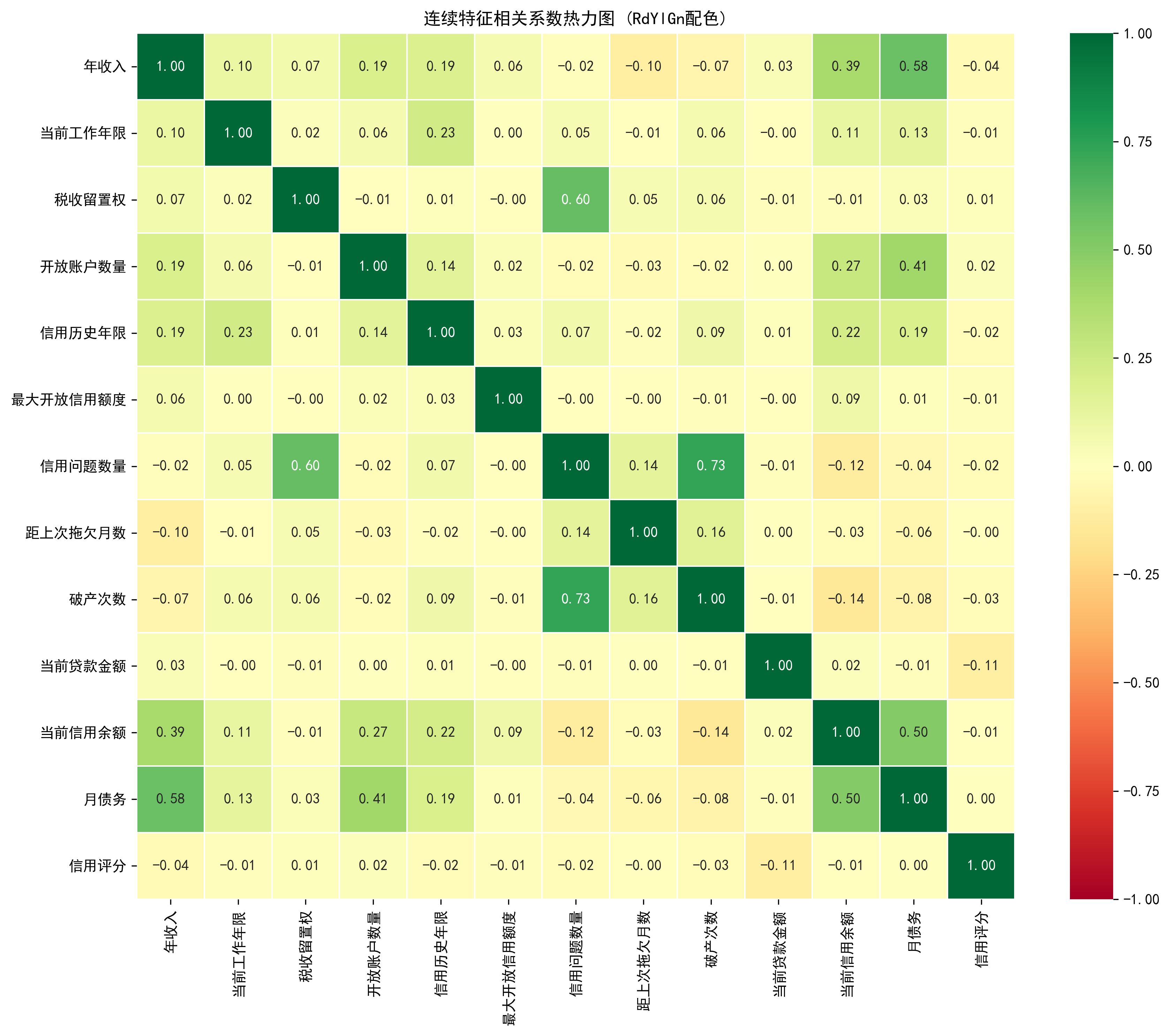
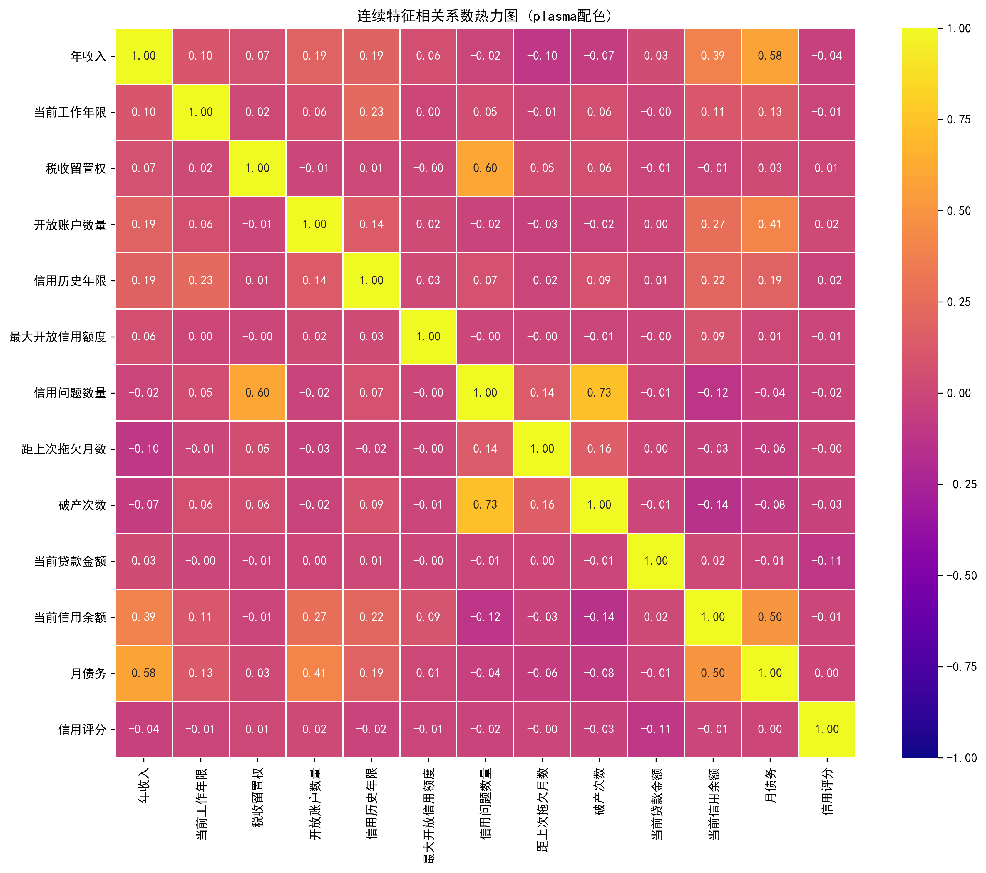
热力图(Heatmap)是一种通过颜色深浅来展示数据矩阵的可视化方法。在数据分析中,我们常用热力图来展示特征之间的相关系数矩阵。
相关系数的含义:
- 取值范围: [-1, 1]
- 接近1: 强正相关(一个增加,另一个也增加)
- 接近-1: 强负相关(一个增加,另一个减少)
- 接近0: 无线性相关关系
注意事项:
- 热力图适合展示连续变量之间的关系
- 对于离散变量,相关系数的意义需要谨慎解读
- 本例中为了演示方便,对所有数值型特征都进行了计算
# 基础热力图 - 使用coolwarm配色
import pandas as pd
import seaborn as sns
import matplotlib.pyplot as plt

# 提取连续值特征(中文名)
continuous_features_cn = [
    '年收入', '当前工作年限', '税收留置权',
    '开放账户数量', '信用历史年限',
    '最大开放信用额度', '信用问题数量',
    '距上次拖欠月数', '破产次数',
    '当前贷款金额', '当前信用余额', '月债务',
    '信用评分'
]

# 计算相关系数矩阵
correlation_matrix = data_cn[continuous_features_cn].corr()

# 设置图片清晰度
plt.rcParams['figure.dpi'] = 300
# 设置中文字体
plt.rcParams['font.sans-serif'] = ['SimHei']  # 用来正常显示中文标签
plt.rcParams['axes.unicode_minus'] = False  # 用来正常显示负号

# 绘制热力图
plt.figure(figsize=(12, 10))
sns.heatmap(correlation_matrix, annot=False, cmap='coolwarm', vmin=-1, vmax=1,
            fmt='.2f', linewidths=0.5)
plt.title('连续特征相关系数热力图 (coolwarm配色)')
plt.tight_layout()
plt.show()

# 使用RdYlGn配色方案
plt.figure(figsize=(12, 10))
sns.heatmap(correlation_matrix, annot=True, cmap='RdYlGn', vmin=-1, vmax=1,
            fmt='.2f', linewidths=0.5, center=0)
plt.title('连续特征相关系数热力图 (RdYlGn配色)')
plt.tight_layout()
plt.show()
# 使用viridis配色方案(色盲友好)
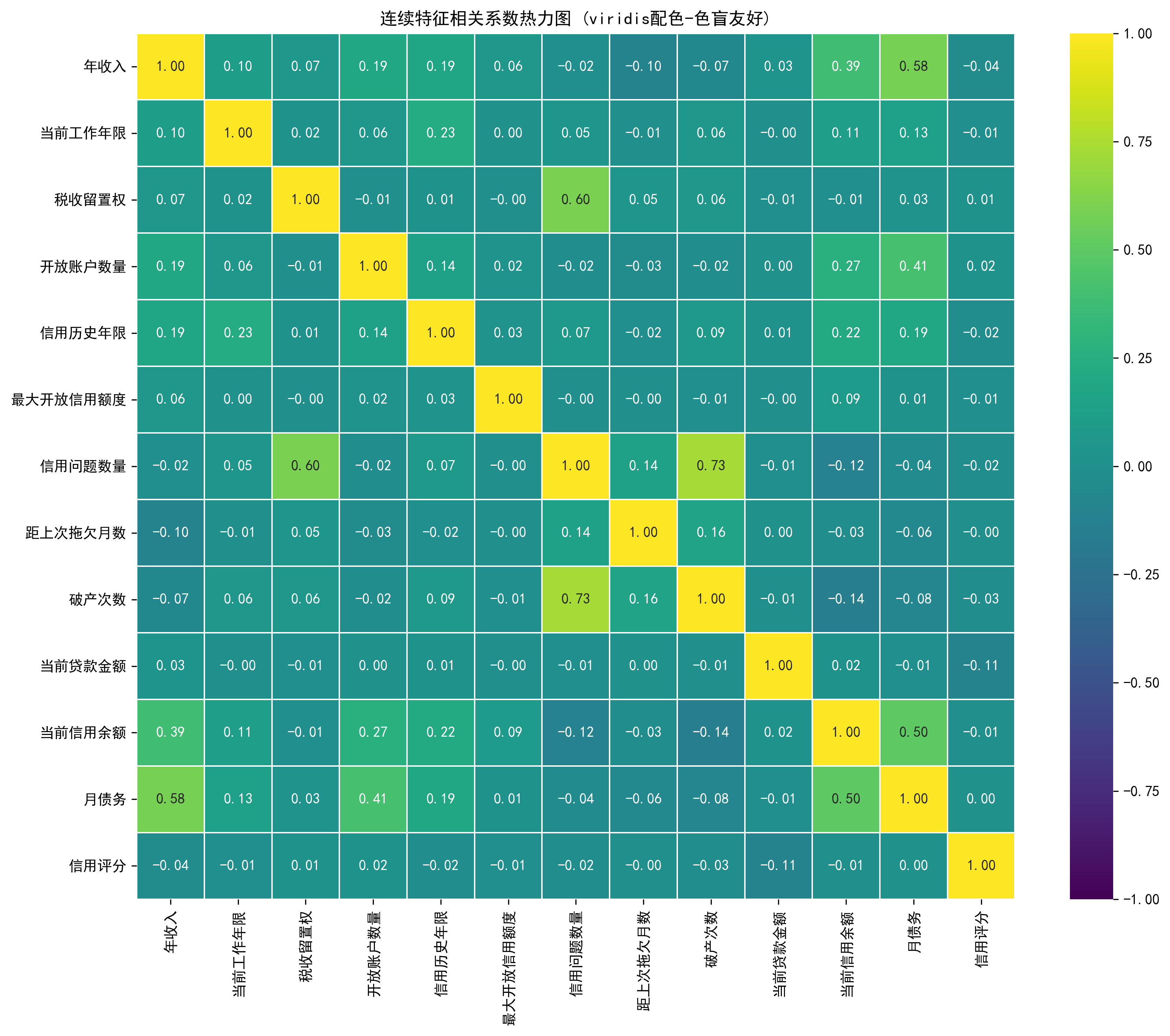
plt.figure(figsize=(12, 10))
sns.heatmap(correlation_matrix, annot=True, cmap='viridis', vmin=-1, vmax=1,
            fmt='.2f', linewidths=0.5)
plt.title('连续特征相关系数热力图 (viridis配色-色盲友好)')
plt.tight_layout()
plt.show()
# 使用plasma配色方案
plt.figure(figsize=(12, 10))
sns.heatmap(correlation_matrix, annot=True, cmap='plasma', vmin=-1, vmax=1,
            fmt='.2f', linewidths=0.5)
plt.title('连续特征相关系数热力图 (plasma配色)')
plt.tight_layout()
plt.show()
# 自定义配色 - 只显示强相关(阈值过滤)
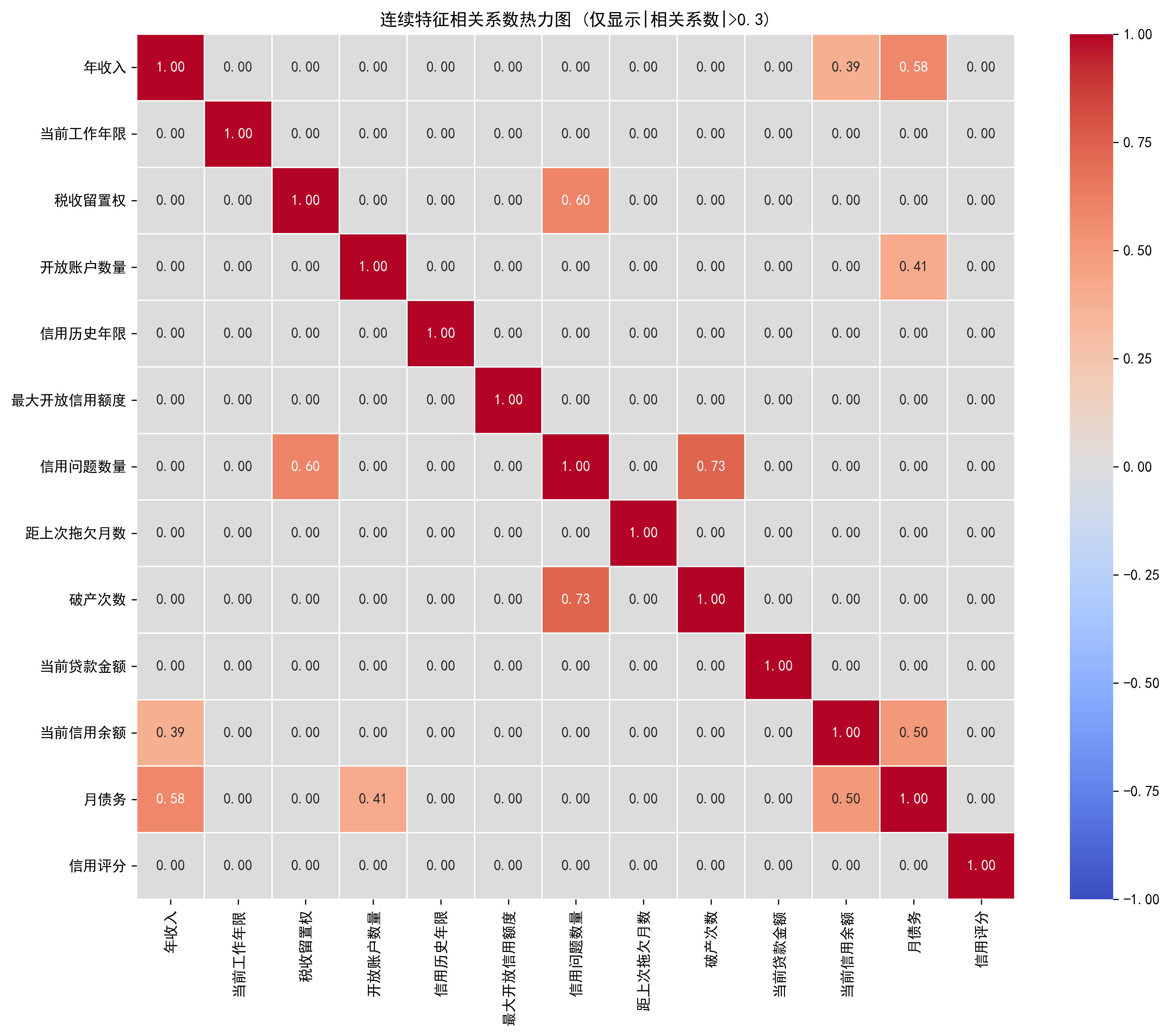
# 创建一个只显示绝对值大于0.3的相关系数矩阵
import numpy as np

correlation_matrix_filtered = correlation_matrix.copy()
correlation_matrix_filtered[np.abs(correlation_matrix_filtered) < 0.3] = 0

plt.figure(figsize=(12, 10))
sns.heatmap(correlation_matrix_filtered, annot=True, cmap='coolwarm', vmin=-1, vmax=1,
            fmt='.2f', linewidths=0.5, center=0)
plt.title('连续特征相关系数热力图 (仅显示|相关系数|>0.3)')
plt.tight_layout()
plt.show()


import numpy as np
import matplotlib.pyplot as plt


# -----------------
# 1. 创建模拟数据
# -----------------
# 子图A的数据:正弦波
X_sin = np.linspace(0, 2 * np.pi, 100)
Y_sin = np.sin(X_sin)

# 子图B的数据:随机散点
X_scatter = np.random.rand(50)
Y_scatter = np.random.rand(50)

# 子图C的数据:条形图
categories = ['A', 'B', 'C', 'D']
values = [15, 30, 10, 25]

# 子图D的数据:线性衰减
X_linear = np.arange(10)
Y_linear = 10 - X_linear * 0.8 + np.random.randn(10) * 0.5


# -----------------
# 2. 绘制子图(核心步骤)
# -----------------

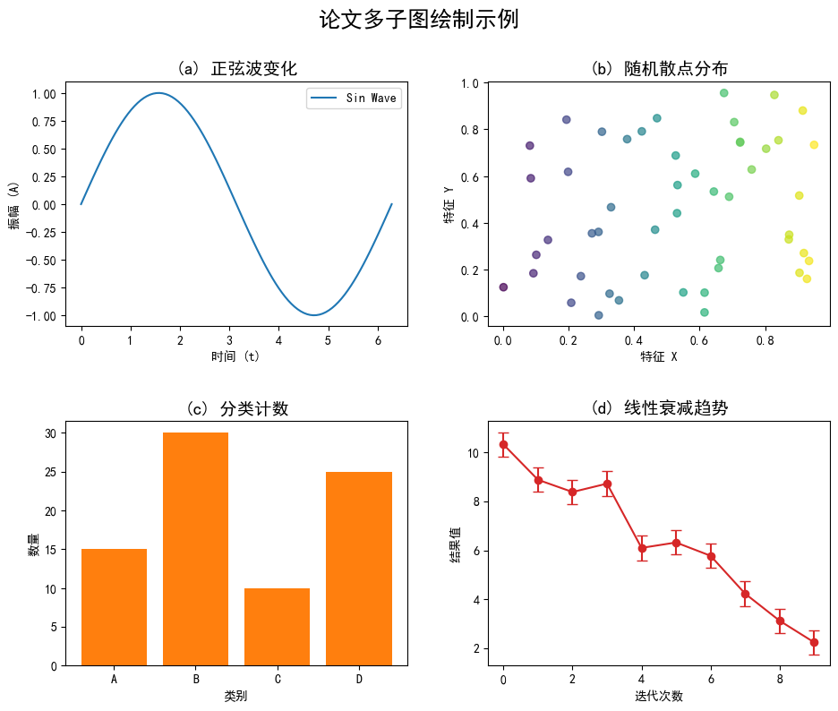
# 使用 plt.subplots() 创建 2x2 的子图布局
# fig: 代表整个画布(Figure)
# axes: 是一个包含所有子图坐标轴对象的 NumPy 数组
fig, axes = plt.subplots(
    nrows=2,           # 行数 (Number of Rows)
    ncols=2,           # 列数 (Number of Columns)
    figsize=(10, 8),   # 整个画布的大小 (10英寸宽, 8英寸高)
    dpi=100            # 分辨率,确保清晰度
)

# -----------------
# 3. 分别在每个子图上绘图和设置属性
# -----------------

# 子图 A (位于第一行第一列:axes[0, 0]) - 绘制折线图
ax_A = axes[0, 0]
ax_A.plot(X_sin, Y_sin, color='tab:blue', label='Sin Wave')
ax_A.set_title('(a) 正弦波变化', fontsize=14, fontweight='bold')
ax_A.set_xlabel('时间 (t)')
ax_A.set_ylabel('振幅 (A)')
ax_A.legend()

# 子图 B (位于第一行第二列:axes[0, 1]) - 绘制散点图
ax_B = axes[0, 1]
ax_B.scatter(X_scatter, Y_scatter, c=X_scatter, cmap='viridis', alpha=0.7)
ax_B.set_title('(b) 随机散点分布', fontsize=14, fontweight='bold')
ax_B.set_xlabel('特征 X')
ax_B.set_ylabel('特征 Y')

# 子图 C (位于第二行第一列:axes[1, 0]) - 绘制条形图
ax_C = axes[1, 0]
ax_C.bar(categories, values, color='tab:orange')
ax_C.set_title('(c) 分类计数', fontsize=14, fontweight='bold')
ax_C.set_xlabel('类别')
ax_C.set_ylabel('数量')

# 子图 D (位于第二行第二列:axes[1, 1]) - 绘制带误差的折线图
ax_D = axes[1, 1]
ax_D.errorbar(X_linear, Y_linear, yerr=0.5, fmt='-o', color='tab:red', capsize=4)
ax_D.set_title('(d) 线性衰减趋势', fontsize=14, fontweight='bold')
ax_D.set_xlabel('迭代次数')
ax_D.set_ylabel('结果值')


# -----------------
# 4. 调整整体布局
# -----------------

# 自动调整子图参数,使之填充整个 figure 区域,避免标签重叠
fig.tight_layout(pad=3.0)

# 给整个画布添加一个总标题
fig.suptitle('论文多子图绘制示例', fontsize=18, fontweight='bold', y=1.02)


# -----------------
# 5. 显示和保存
# -----------------
plt.show()

# 如果要保存高质量图片,建议使用矢量格式,例如:
# fig.savefig('my_subplots.pdf', format='pdf', bbox_inches='tight')
# fig.savefig('my_subplots.png', dpi=300) # 位图保存
# enumerate()函数示例
fruits = ['苹果', '香蕉', '橙子', '葡萄']

# 不使用enumerate - 需要手动维护索引
print("不使用enumerate:")
index = 0
for fruit in fruits:
    print(f"索引 {index}: {fruit}")
    index += 1
不使用enumerate:
索引 0: 苹果
索引 1: 香蕉
索引 2: 橙子
索引 3: 葡萄
print("\n使用enumerate:")
# 使用enumerate - 自动获取索引
for index, fruit in enumerate(fruits):
    print(f"索引 {index}: {fruit}")
使用enumerate:
索引 0: 苹果
索引 1: 香蕉
索引 2: 橙子
索引 3: 葡萄
print("\n从1开始计数:")
# enumerate还可以指定起始索引
for index, fruit in enumerate(fruits, start=1):
    print(f"第 {index} 个水果: {fruit}")
从1开始计数:
第 1 个水果: 苹果
第 2 个水果: 香蕉
第 3 个水果: 橙子
第 4 个水果: 葡萄

# 提取连续变量列表(使用中文名)
continuous_features_cn = [
    '年收入', '当前工作年限', '税收留置权',
    '开放账户数量', '信用历史年限',
    '最大开放信用额度', '信用问题数量',
    '距上次拖欠月数', '破产次数',
    '当前贷款金额', '当前信用余额', '月债务',
    '信用评分'
]

# 计算需要多少行和列
n_features = len(continuous_features_cn)
n_cols = 3  # 每行显示3个图
n_rows = (n_features + n_cols - 1) // n_cols  # 向上取整计算需要的行数

# 创建子图
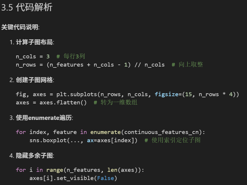
fig, axes = plt.subplots(n_rows, n_cols, figsize=(15, n_rows * 4))
# 将axes展平为一维数组,方便使用索引访问
axes = axes.flatten()

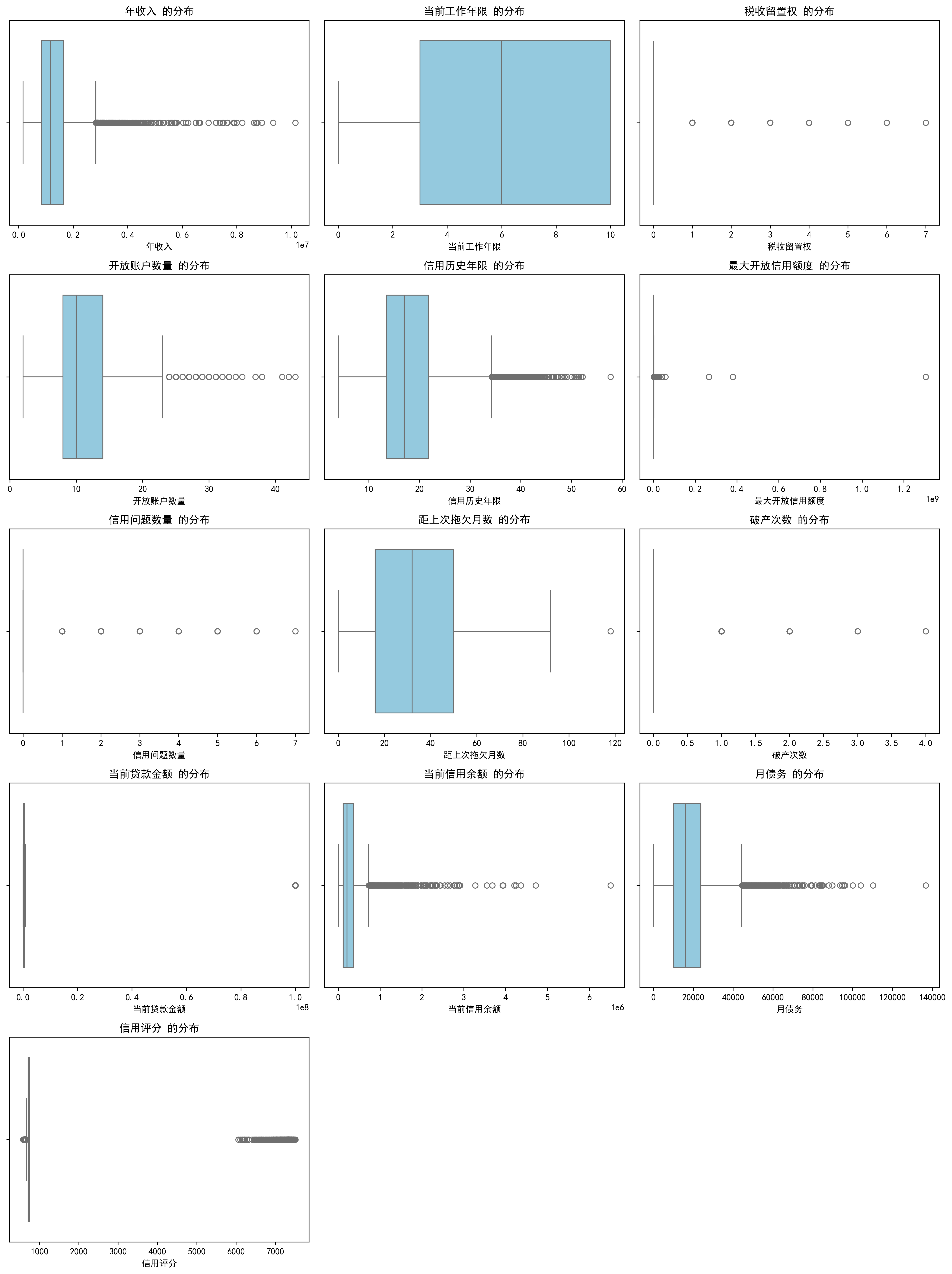
# 遍历每个连续变量,绘制箱线图
for index, feature in enumerate(continuous_features_cn):
    # 在第index个子图上绘制
    sns.boxplot(x=data_cn[feature], ax=axes[index], color='skyblue')
    axes[index].set_title(f'{feature} 的分布', fontsize=12, fontweight='bold')
    axes[index].set_xlabel(feature, fontsize=10)

# 隐藏多余的空白子图
for i in range(n_features, len(axes)):
    axes[i].set_visible(False)

plt.tight_layout()
plt.show()

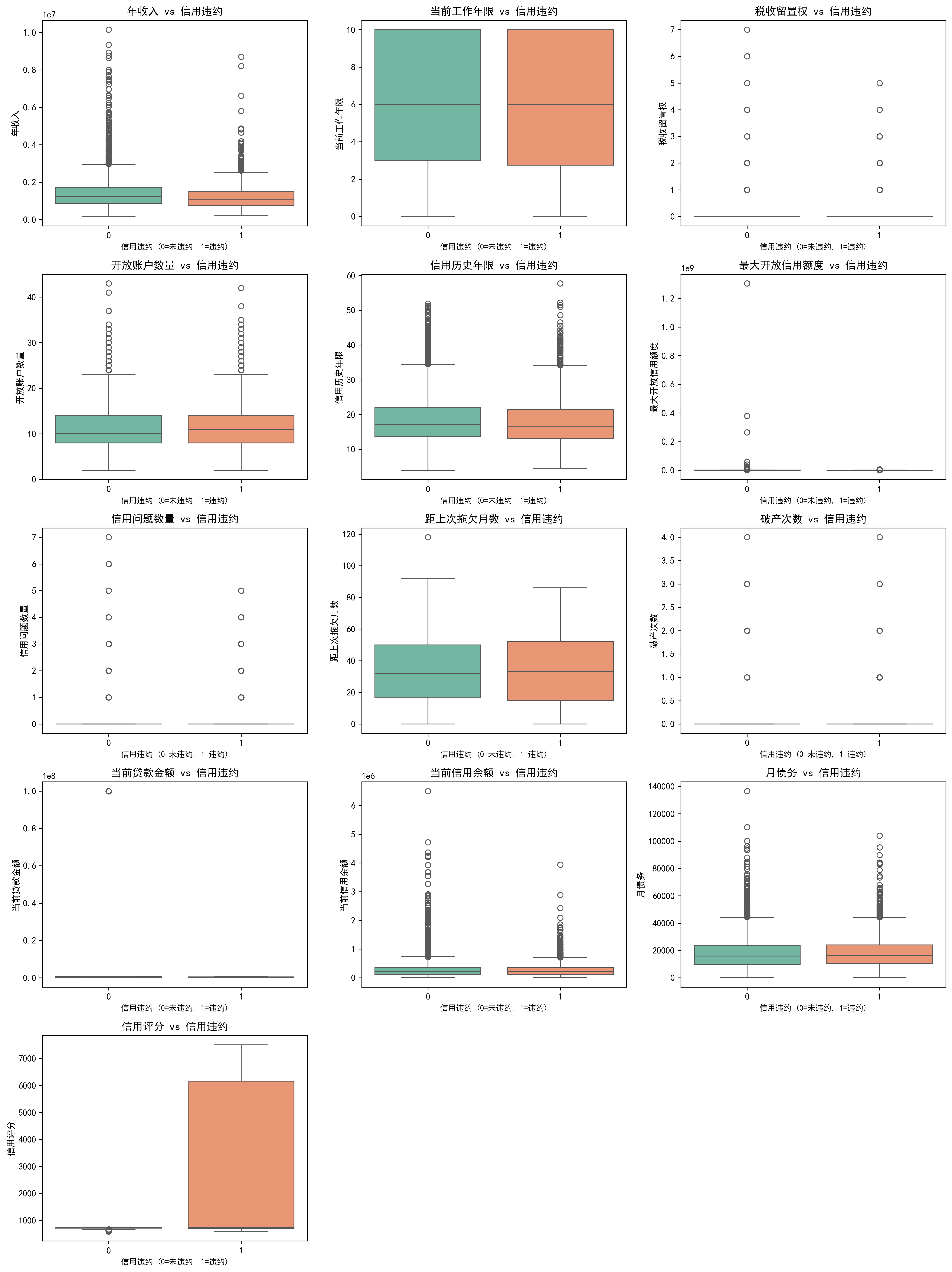
# 创建按信用违约分组的箱线图
fig, axes = plt.subplots(n_rows, n_cols, figsize=(15, n_rows * 4))
axes = axes.flatten()

# 遍历每个连续变量
for index, feature in enumerate(continuous_features_cn):
    # 在第index个子图上绘制,按信用违约分组
    sns.boxplot(x='信用违约', y=feature, data=data_cn, ax=axes[index], palette='Set2')
    axes[index].set_title(f'{feature} vs 信用违约', fontsize=12, fontweight='bold')
    axes[index].set_xlabel('信用违约 (0=未违约, 1=违约)', fontsize=9)
    axes[index].set_ylabel(feature, fontsize=10)

# 隐藏多余的空白子图
for i in range(n_features, len(axes)):
    axes[i].set_visible(False)

plt.tight_layout()
plt.show()
今天的文章有点长,希望能耐心看完,前面示教的包括:enumerate()、嵌套字典、特征与处理过程都是我们前面的课中间学到的。所以要理解的实际上很少,加油!!
更多推荐

 33
33 0
0- 0


 已为社区贡献11条内容

所有评论(0)