
机器学习与深度学习day10——机器学习建模与评估
DAY10
前言:
我们这节课的题目是ML模型的建模与评估,但是我们实际上的流程是:
数据预处理→导库(选模型与指标)→训练模型(三行经典代码)→评估(选评估指标)
实际上,我们训练第一个模型时候,就已经结束了,待会儿大家看代码就知道了,全文手敲,熟悉流程了以后,用ai就很方便了。
- 把之前所有的处理手段都处理一遍,回顾一下全流程,以后就用处理好的部分直接完成
- 开始机器学习建模(简单建模,不涉及调参)和评估
一、数据预处理
1.1 导入所需要的包
这里其实是写完后一起整理到这里的
import pandas as pd
import pandas as pd    #用于数据处理和分析,可处理表格数据。
import numpy as np     #用于数值计算,提供了高效的数组操作。
import matplotlib.pyplot as plt    #用于绘制各种类型的图表
import seaborn as sns   #基于matplotlib的高级绘图库,能绘制更美观的统计图形。
import warnings
warnings.filterwarnings('ignore')

 # 设置中文字体(解决中文显示问题)
plt.rcParams['font.sans-serif'] = ['SimHei']  # Windows系统常用黑体字体
plt.rcParams['axes.unicode_minus'] = False    # 正常显示负号
1.2 查看数据信息
data = pd.read_csv('data.csv') #读取数据
data.head()
| Id | Home Ownership | Annual Income | Years in current job | Tax Liens | Number of Open Accounts | Years of Credit History | Maximum Open Credit | Number of Credit Problems | Months since last delinquent | Bankruptcies | Purpose | Term | Current Loan Amount | Current Credit Balance | Monthly Debt | Credit Score | Credit Default | |
|---|---|---|---|---|---|---|---|---|---|---|---|---|---|---|---|---|---|---|
| 0 | 0 | Own Home | 482087.0 | NaN | 0.0 | 11.0 | 26.3 | 685960.0 | 1.0 | NaN | 1.0 | debt consolidation | Short Term | 99999999.0 | 47386.0 | 7914.0 | 749.0 | 0 |
| 1 | 1 | Own Home | 1025487.0 | 10+ years | 0.0 | 15.0 | 15.3 | 1181730.0 | 0.0 | NaN | 0.0 | debt consolidation | Long Term | 264968.0 | 394972.0 | 18373.0 | 737.0 | 1 |
| 2 | 2 | Home Mortgage | 751412.0 | 8 years | 0.0 | 11.0 | 35.0 | 1182434.0 | 0.0 | NaN | 0.0 | debt consolidation | Short Term | 99999999.0 | 308389.0 | 13651.0 | 742.0 | 0 |
| 3 | 3 | Own Home | 805068.0 | 6 years | 0.0 | 8.0 | 22.5 | 147400.0 | 1.0 | NaN | 1.0 | debt consolidation | Short Term | 121396.0 | 95855.0 | 11338.0 | 694.0 | 0 |
| 4 | 4 | Rent | 776264.0 | 8 years | 0.0 | 13.0 | 13.6 | 385836.0 | 1.0 | NaN | 0.0 | debt consolidation | Short Term | 125840.0 | 93309.0 | 7180.0 | 719.0 | 0 |
1.3 特征名映射
# 创建特征名中文映射字典
feature_name_mapping = {
    'Annual Income': '年收入',
    'Years in current job': '当前工作年限',
    'Tax Liens': '税收留置权',
    'Number of Open Accounts': '开放账户数量',
    'Years of Credit History': '信用历史年限',
    'Maximum Open Credit': '最大开放信用额度',
    'Number of Credit Problems': '信用问题数量',
    'Months since last delinquent': '距上次拖欠月数',
    'Bankruptcies': '破产次数',
    'Current Loan Amount': '当前贷款金额',
    'Current Credit Balance': '当前信用余额',
    'Monthly Debt': '月债务',
    'Credit Score': '信用评分',
    'Home Ownership': '房屋所有权',
    'Term': '贷款期限',
    'Purpose': '贷款目的',
    'Credit Default': '信用违约'
}

# 重命名数据框的列名
data = data.rename(columns=feature_name_mapping)
data.head()
| Id | 房屋所有权 | 年收入 | 当前工作年限 | 税收留置权 | 开放账户数量 | 信用历史年限 | 最大开放信用额度 | 信用问题数量 | 距上次拖欠月数 | 破产次数 | 贷款目的 | 贷款期限 | 当前贷款金额 | 当前信用余额 | 月债务 | 信用评分 | 信用违约 | |
|---|---|---|---|---|---|---|---|---|---|---|---|---|---|---|---|---|---|---|
| 0 | 0 | Own Home | 482087.0 | NaN | 0.0 | 11.0 | 26.3 | 685960.0 | 1.0 | NaN | 1.0 | debt consolidation | Short Term | 99999999.0 | 47386.0 | 7914.0 | 749.0 | 0 |
| 1 | 1 | Own Home | 1025487.0 | 10+ years | 0.0 | 15.0 | 15.3 | 1181730.0 | 0.0 | NaN | 0.0 | debt consolidation | Long Term | 264968.0 | 394972.0 | 18373.0 | 737.0 | 1 |
| 2 | 2 | Home Mortgage | 751412.0 | 8 years | 0.0 | 11.0 | 35.0 | 1182434.0 | 0.0 | NaN | 0.0 | debt consolidation | Short Term | 99999999.0 | 308389.0 | 13651.0 | 742.0 | 0 |
| 3 | 3 | Own Home | 805068.0 | 6 years | 0.0 | 8.0 | 22.5 | 147400.0 | 1.0 | NaN | 1.0 | debt consolidation | Short Term | 121396.0 | 95855.0 | 11338.0 | 694.0 | 0 |
| 4 | 4 | Rent | 776264.0 | 8 years | 0.0 | 13.0 | 13.6 | 385836.0 | 1.0 | NaN | 0.0 | debt consolidation | Short Term | 125840.0 | 93309.0 | 7180.0 | 719.0 | 0 |
1.4 删除无用列
# 删除无用列,如ID列
data = data.drop(columns=['Id'])
data.head()
| 房屋所有权 | 年收入 | 当前工作年限 | 税收留置权 | 开放账户数量 | 信用历史年限 | 最大开放信用额度 | 信用问题数量 | 距上次拖欠月数 | 破产次数 | 贷款目的 | 贷款期限 | 当前贷款金额 | 当前信用余额 | 月债务 | 信用评分 | 信用违约 | |
|---|---|---|---|---|---|---|---|---|---|---|---|---|---|---|---|---|---|
| 0 | Own Home | 482087.0 | NaN | 0.0 | 11.0 | 26.3 | 685960.0 | 1.0 | NaN | 1.0 | debt consolidation | Short Term | 99999999.0 | 47386.0 | 7914.0 | 749.0 | 0 |
| 1 | Own Home | 1025487.0 | 10+ years | 0.0 | 15.0 | 15.3 | 1181730.0 | 0.0 | NaN | 0.0 | debt consolidation | Long Term | 264968.0 | 394972.0 | 18373.0 | 737.0 | 1 |
| 2 | Home Mortgage | 751412.0 | 8 years | 0.0 | 11.0 | 35.0 | 1182434.0 | 0.0 | NaN | 0.0 | debt consolidation | Short Term | 99999999.0 | 308389.0 | 13651.0 | 742.0 | 0 |
| 3 | Own Home | 805068.0 | 6 years | 0.0 | 8.0 | 22.5 | 147400.0 | 1.0 | NaN | 1.0 | debt consolidation | Short Term | 121396.0 | 95855.0 | 11338.0 | 694.0 | 0 |
| 4 | Rent | 776264.0 | 8 years | 0.0 | 13.0 | 13.6 | 385836.0 | 1.0 | NaN | 0.0 | debt consolidation | Short Term | 125840.0 | 93309.0 | 7180.0 | 719.0 | 0 |
1.5 编码映射
先打印看一下可能有问题的几个特征的分布,分别是房屋所有权、当前工作年限、贷款目的、贷款期限
这里我们没有再用根据变量类型来筛选的方法了,因为那样很粗糙,我们实际上肯定要理解数据的
# 先打印看一下可能有问题的几个特征的分布,分别是房屋所有权、当前工作年限、贷款目的、贷款期限
print(data['房屋所有权'].value_counts())
房屋所有权
Home Mortgage    3637
Rent             3204
Own Home          647
Have Mortgage      12
Name: count, dtype: int64
# 对房屋所有权进行映射
mappings = {
    "房屋所有权": {
        "Rent": 0, # 租房
        "Have Mortgage": 1, # 有房贷
        "Home Mortgage": 1, # 有房贷
        "Own Home": 2, # 自有住房
    }
}
data = data.replace(mappings)
data['房屋所有权'].value_counts()
房屋所有权
1    3649
0    3204
2     647
Name: count, dtype: int64
print(data['当前工作年限'].value_counts())
当前工作年限
10+ years    2332
2 years       705
3 years       620
< 1 year      563
5 years       516
1 year        504
4 years       469
6 years       426
7 years       396
8 years       339
9 years       259
Name: count, dtype: int64
# 对当前工作年限进行映射
work_year_mappings = {
    "当前工作年限": {
        "< 1 year": 0,
        "1 year": 1,
        "2 years": 2,
        "3 years": 3,
        "4 years": 4,
        "5 years": 5,
        "6 years": 6,
        "7 years": 7,
        "8 years": 8,
        "9 years": 9,
        "10+ years": 10
    }
}
data = data.replace(work_year_mappings)
data['当前工作年限'].value_counts()
当前工作年限
10.0    2332
2.0      705
3.0      620
0.0      563
5.0      516
1.0      504
4.0      469
6.0      426
7.0      396
8.0      339
9.0      259
Name: count, dtype: int64
print(data['贷款目的'].value_counts())
贷款目的
debt consolidation      5944
other                    665
home improvements        412
business loan            129
buy a car                 96
medical bills             71
major purchase            40
take a trip               37
buy house                 34
small business            26
wedding                   15
moving                    11
educational expenses      10
vacation                   8
renewable energy           2
Name: count, dtype: int64
贷款目的是一个需要独热编码的特征,这里为了方便,我们还是沿用便签编码了-----法无定则
注意我们之前说了,如果独热编码的话,就需要先填补缺失值,再独热编码比较合适
# 根据 value_counts() 频率顺序定义映射字典
purpose_ordinal_map = {
    "debt consolidation": 0,
    "other": 1,
    "home improvements": 2,
    "business loan": 3,
    "buy a car": 4,
    "medical bills": 5,
    "major purchase": 6,
    "take a trip": 7,
    "buy house": 8,
    "small business": 9,
    "wedding": 10,
    "moving": 11,
    "educational expenses": 12,
    "vacation": 13,
    "renewable energy": 14
}

# 直接替换原列
data['贷款目的'] = data['贷款目的'].replace(purpose_ordinal_map)

print(data['贷款目的'].value_counts())
贷款目的
0     5944
1      665
2      412
3      129
4       96
5       71
6       40
7       37
8       34
9       26
10      15
11      11
12      10
13       8
14       2
Name: count, dtype: int64
print(data['贷款期限'].value_counts())
贷款期限
Short Term    5556
Long Term     1944
Name: count, dtype: int64
# 对贷款期限进行映射
term_mapping = {
        "Short Term": 0,
        "Long Term": 1
}
data['贷款期限'] = data['贷款期限'].replace(term_mapping)
data['贷款期限'].value_counts()
贷款期限
0    5556
1    1944
Name: count, dtype: int64
data.head()
| 房屋所有权 | 年收入 | 当前工作年限 | 税收留置权 | 开放账户数量 | 信用历史年限 | 最大开放信用额度 | 信用问题数量 | 距上次拖欠月数 | 破产次数 | 贷款目的 | 贷款期限 | 当前贷款金额 | 当前信用余额 | 月债务 | 信用评分 | 信用违约 | |
|---|---|---|---|---|---|---|---|---|---|---|---|---|---|---|---|---|---|
| 0 | 2 | 482087.0 | NaN | 0.0 | 11.0 | 26.3 | 685960.0 | 1.0 | NaN | 1.0 | 0 | 0 | 99999999.0 | 47386.0 | 7914.0 | 749.0 | 0 |
| 1 | 2 | 1025487.0 | 10.0 | 0.0 | 15.0 | 15.3 | 1181730.0 | 0.0 | NaN | 0.0 | 0 | 1 | 264968.0 | 394972.0 | 18373.0 | 737.0 | 1 |
| 2 | 1 | 751412.0 | 8.0 | 0.0 | 11.0 | 35.0 | 1182434.0 | 0.0 | NaN | 0.0 | 0 | 0 | 99999999.0 | 308389.0 | 13651.0 | 742.0 | 0 |
| 3 | 2 | 805068.0 | 6.0 | 0.0 | 8.0 | 22.5 | 147400.0 | 1.0 | NaN | 1.0 | 0 | 0 | 121396.0 | 95855.0 | 11338.0 | 694.0 | 0 |
| 4 | 0 | 776264.0 | 8.0 | 0.0 | 13.0 | 13.6 | 385836.0 | 1.0 | NaN | 0.0 | 0 | 0 | 125840.0 | 93309.0 | 7180.0 | 719.0 | 0 |
现在已经没有非数值类型的特征了
data.info()
<class 'pandas.core.frame.DataFrame'>
RangeIndex: 7500 entries, 0 to 7499
Data columns (total 17 columns):
 #   Column    Non-Null Count  Dtype
---  ------    --------------  -----
 0   房屋所有权     7500 non-null   int64
 1   年收入       5943 non-null   float64
 2   当前工作年限    7129 non-null   float64
 3   税收留置权     7500 non-null   float64
 4   开放账户数量    7500 non-null   float64
 5   信用历史年限    7500 non-null   float64
 6   最大开放信用额度  7500 non-null   float64
 7   信用问题数量    7500 non-null   float64
 8   距上次拖欠月数   3419 non-null   float64
 9   破产次数      7486 non-null   float64
 10  贷款目的      7500 non-null   int64
 11  贷款期限      7500 non-null   int64
 12  当前贷款金额    7500 non-null   float64
 13  当前信用余额    7500 non-null   float64
 14  月债务       7500 non-null   float64
 15  信用评分      5943 non-null   float64
 16  信用违约      7500 non-null   int64
dtypes: float64(13), int64(4)
memory usage: 996.2 KB
1.6 填补缺失值
# 确定需要填充的列
missing_cols = [
    '年收入',
    '当前工作年限',
    '距上次拖欠月数',
    '破产次数',
    '信用评分'
]

print("开始使用众数(Mode)填充缺失值...")

for col in missing_cols:
    # 计算众数。由于可能存在多个众数,.mode() 返回 Series,我们取第一个 [0]
    mode_val = data[col].mode()[0]

    # 使用众数填充缺失值
    data[col].fillna(mode_val, inplace=True)

    print(f"列 '{col}' 已使用众数 {mode_val} 填充。")

# 验证处理结果
print("\n--- 缺失值处理后的 DataFrame 信息 ---")
data.info()
开始使用众数(Mode)填充缺失值...
列 '年收入' 已使用众数 969475.0 填充。
列 '当前工作年限' 已使用众数 10.0 填充。
列 '距上次拖欠月数' 已使用众数 14.0 填充。
列 '破产次数' 已使用众数 0.0 填充。
列 '信用评分' 已使用众数 740.0 填充。

--- 缺失值处理后的 DataFrame 信息 ---
<class 'pandas.core.frame.DataFrame'>
RangeIndex: 7500 entries, 0 to 7499
Data columns (total 17 columns):
 #   Column    Non-Null Count  Dtype
---  ------    --------------  -----
 0   房屋所有权     7500 non-null   int64
 1   年收入       7500 non-null   float64
 2   当前工作年限    7500 non-null   float64
 3   税收留置权     7500 non-null   float64
 4   开放账户数量    7500 non-null   float64
 5   信用历史年限    7500 non-null   float64
 6   最大开放信用额度  7500 non-null   float64
 7   信用问题数量    7500 non-null   float64
 8   距上次拖欠月数   7500 non-null   float64
 9   破产次数      7500 non-null   float64
 10  贷款目的      7500 non-null   int64
 11  贷款期限      7500 non-null   int64
 12  当前贷款金额    7500 non-null   float64
 13  当前信用余额    7500 non-null   float64
 14  月债务       7500 non-null   float64
 15  信用评分      7500 non-null   float64
 16  信用违约      7500 non-null   int64
dtypes: float64(13), int64(4)
memory usage: 996.2 KB
1.7 异常值处理
- 我们之前没说异常值的处理,实际上是可处理可不处理的,因为这需要考验你对于实际数据的理解,而且不处理也会增强泛化性和鲁棒性,因为实际中很多收上来的数据本身就有问题
- 异常值一般不处理,或者结合对照试验处理和不处理都尝试下,但是论文中要写这个,作为工作量
data.head()
| 房屋所有权 | 年收入 | 当前工作年限 | 税收留置权 | 开放账户数量 | 信用历史年限 | 最大开放信用额度 | 信用问题数量 | 距上次拖欠月数 | 破产次数 | 贷款目的 | 贷款期限 | 当前贷款金额 | 当前信用余额 | 月债务 | 信用评分 | 信用违约 | |
|---|---|---|---|---|---|---|---|---|---|---|---|---|---|---|---|---|---|
| 0 | 2 | 482087.0 | 10.0 | 0.0 | 11.0 | 26.3 | 685960.0 | 1.0 | 14.0 | 1.0 | 0 | 0 | 99999999.0 | 47386.0 | 7914.0 | 749.0 | 0 |
| 1 | 2 | 1025487.0 | 10.0 | 0.0 | 15.0 | 15.3 | 1181730.0 | 0.0 | 14.0 | 0.0 | 0 | 1 | 264968.0 | 394972.0 | 18373.0 | 737.0 | 1 |
| 2 | 1 | 751412.0 | 8.0 | 0.0 | 11.0 | 35.0 | 1182434.0 | 0.0 | 14.0 | 0.0 | 0 | 0 | 99999999.0 | 308389.0 | 13651.0 | 742.0 | 0 |
| 3 | 2 | 805068.0 | 6.0 | 0.0 | 8.0 | 22.5 | 147400.0 | 1.0 | 14.0 | 1.0 | 0 | 0 | 121396.0 | 95855.0 | 11338.0 | 694.0 | 0 |
| 4 | 0 | 776264.0 | 8.0 | 0.0 | 13.0 | 13.6 | 385836.0 | 1.0 | 14.0 | 0.0 | 0 | 0 | 125840.0 | 93309.0 | 7180.0 | 719.0 | 0 |
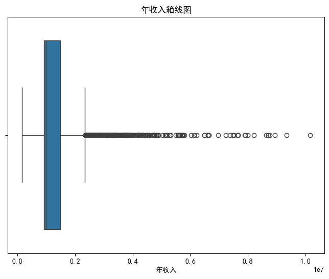
这里我们选择年收入来处理吧,我们选择四分位数范围 (IQR),他是基于箱线图原理来定义异常值边界
# 绘制年收入的箱线图
plt.figure(figsize=(8, 6))
sns.boxplot(x=data['年收入'])
plt.title('年收入箱线图')
plt.xlabel('年收入')
plt.show()
column_name = '年收入'

# 1. 计算 Q1, Q3 和 IQR
Q1 = data[column_name].quantile(0.25)
Q3 = data[column_name].quantile(0.75)
IQR = Q3 - Q1

# 2. 确定异常值边界 (使用 1.5 倍 IQR)
lower_bound = Q1 - 1.5 * IQR
upper_bound = Q3 + 1.5 * IQR

print(f"--- '{column_name}' 异常值处理信息 ---")
print(f"Q1 (25th Percentile): {Q1:.2f}")
print(f"Q3 (75th Percentile): {Q3:.2f}")
print(f"IQR (Q3 - Q1): {IQR:.2f}")
print(f"下限 (Lower Bound): {lower_bound:.2f}")
print(f"上限 (Upper Bound): {upper_bound:.2f}")

# 3. 筛选数据:保留在边界内的数据
data_before_drop = len(data)
data_filtered = data[
    (data[column_name] >= lower_bound) &
    (data[column_name] <= upper_bound)
].copy() # 使用 .copy() 避免 SettingWithCopyWarning

# 4. 更新 DataFrame 并报告结果
data = data_filtered
data_after_drop = len(data)
rows_dropped = data_before_drop - data_after_drop

print(f"\n原始数据行数: {data_before_drop}")
print(f"删除异常值后行数: {data_after_drop}")
print(f"共删除异常值 (行): {rows_dropped}")

print(f"\nDataFrame 已更新,'{column_name}' 的异常值已被移除。")
--- '年收入' 异常值处理信息 ---
Q1 (25th Percentile): 931133.00
Q3 (75th Percentile): 1499974.00
IQR (Q3 - Q1): 568841.00
下限 (Lower Bound): 77871.50
上限 (Upper Bound): 2353235.50

原始数据行数: 7500
删除异常值后行数: 6984
共删除异常值 (行): 516

DataFrame 已更新,'年收入' 的异常值已被移除。
# 绘制年收入的箱线图
plt.figure(figsize=(8, 6))
sns.boxplot(x=data['年收入'])
plt.title('年收入箱线图')
plt.xlabel('年收入')
plt.show()
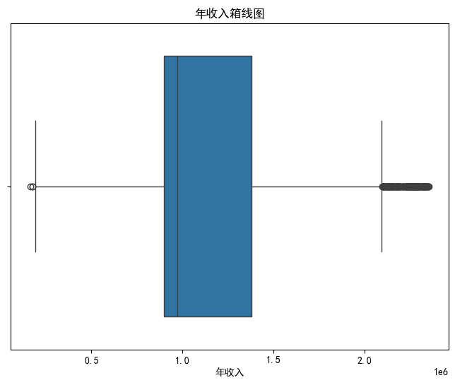
为什么删除了异常值后箱线图上还是有点? 这是因为箱线图是一个“递归”的概念,每次您移除异常值并重新绘制时,箱体和边界都会重新计算。
- 每次对新数据 q1和q3都会重新计算,所以上下限会重新计算
- 但是即使如此,新的箱线图会分布更加集中
解决这个问题直接设置好固定上限即可
data.info()
<class 'pandas.core.frame.DataFrame'>
Index: 6984 entries, 0 to 7499
Data columns (total 17 columns):
 #   Column    Non-Null Count  Dtype
---  ------    --------------  -----
 0   房屋所有权     6984 non-null   int64
 1   年收入       6984 non-null   float64
 2   当前工作年限    6984 non-null   float64
 3   税收留置权     6984 non-null   float64
 4   开放账户数量    6984 non-null   float64
 5   信用历史年限    6984 non-null   float64
 6   最大开放信用额度  6984 non-null   float64
 7   信用问题数量    6984 non-null   float64
 8   距上次拖欠月数   6984 non-null   float64
 9   破产次数      6984 non-null   float64
 10  贷款目的      6984 non-null   int64
 11  贷款期限      6984 non-null   int64
 12  当前贷款金额    6984 non-null   float64
 13  当前信用余额    6984 non-null   float64
 14  月债务       6984 non-null   float64
 15  信用评分      6984 non-null   float64
 16  信用违约      6984 non-null   int64
dtypes: float64(13), int64(4)
memory usage: 982.1 KB
可以看到,删除异常值是删除了所有的样本,也可以只删除这个特征值而不删除整个样本,再用缺失值填补即可。
1.8 可视化分析
这部分不在赘述,3类图,自行选择
1.9 其他核心部分
特征工程
- 衍生新特征:根据已有特征创建新的特征,可能会对模型性能有提升。例如,可以计算“Debt - to - Income Ratio”(负债收入比),即“Monthly Debt”与“Annual Income”的比值,来反映客户的债务负担情况。
- 特征选择:通过相关性分析等方法,选择与目标变量“Credit Default”相关性较高的特征,去除相关性较低或冗余的特征,以降低模型的复杂度和过拟合的风险。
此外,数据不平衡输出我们后面再说
此时你可能会好奇,怎么还没有归一化/标准化?这就需要我们引入数据泄露的观点了
我们之所以推迟归一化或标准化步骤,正是为了避免关键的训练集/测试集数据泄露问题。一旦在划分数据集之前对全集应用此类预处理,训练过程就间接利用了测试集的均值和标准差等统计信息,这会导致对模型在未知数据上性能的乐观估计。课上反复提及的核心:
考试理论:
- 不要提前知道考试题。
- 调参就需要考2次
二、机器学习模型建模
2.1 数据划分
data.columns
Index(['房屋所有权', '年收入', '当前工作年限', '税收留置权', '开放账户数量', '信用历史年限', '最大开放信用额度',
       '信用问题数量', '距上次拖欠月数', '破产次数', '贷款目的', '贷款期限', '当前贷款金额', '当前信用余额', '月债务',
       '信用评分', '信用违约'],
      dtype='object')
# 划分训练集和测试集
from sklearn.model_selection import train_test_split
X = data.drop(['信用违约'], axis=1)  # 特征,axis=1表示按列删除
y = data['信用违约']  # 标签
X_train, X_test, y_train, y_test = train_test_split(X, y, test_size=0.2, random_state=42)  # 划分数据集,20%作为测试集,随机种子为42
# 训练集和测试集的形状
print(f"训练集形状: {X_train.shape}, 测试集形状: {X_test.shape}")  # 打印训练集和测试集的形状
训练集形状: (5587, 16), 测试集形状: (1397, 16)
2.2 数据归一化
只需要对连续特征归一化即可,离散特征编码后虽然是数值,但是不用动
from sklearn.model_selection import train_test_split
from sklearn.preprocessing import StandardScaler, MinMaxScaler

# ----------------------------------------------------------------------
# 定义连续特征列 (需要归一化的特征)
# ----------------------------------------------------------------------
continuous_features = [
    '年收入',
    '当前工作年限',
    '开放账户数量', # 虽为计数,但一般也进行缩放
    '信用历史年限',
    '最大开放信用额度',
    '距上次拖欠月数',
    '当前贷款金额',
    '当前信用余额',
    '月债务',
    '信用评分'
]

# 初始化归一化器 (MinMaxScaler)
scaler = MinMaxScaler()


# 仅在训练集上 fit (学习最大值和最小值)
# 然后对训练集进行 transform (应用缩放)
# 注意:Scikit-learn 返回 NumPy 数组,需要重新赋值给 DataFrame
X_train[continuous_features] = scaler.fit_transform(X_train[continuous_features])

# 使用训练集学到的参数 (scaler) 直接对测试集进行 transform
# 绝对不能对测试集使用 fit_transform()
X_test[continuous_features] = scaler.transform(X_test[continuous_features])
X_test
| 房屋所有权 | 年收入 | 当前工作年限 | 税收留置权 | 开放账户数量 | 信用历史年限 | 最大开放信用额度 | 信用问题数量 | 距上次拖欠月数 | 破产次数 | 贷款目的 | 贷款期限 | 当前贷款金额 | 当前信用余额 | 月债务 | 信用评分 | |
|---|---|---|---|---|---|---|---|---|---|---|---|---|---|---|---|---|
| 3161 | 1 | 0.399142 | 0.7 | 0.0 | 0.300 | 0.409683 | 0.000378 | 0.0 | 0.315217 | 0.0 | 0 | 1 | 0.005110 | 0.092358 | 0.289425 | 0.007220 |
| 4119 | 1 | 0.363551 | 0.2 | 0.0 | 0.200 | 0.189944 | 0.000000 | 0.0 | 0.152174 | 0.0 | 0 | 1 | 0.002002 | 0.000000 | 0.074997 | 0.022238 |
| 4317 | 0 | 0.283759 | 0.2 | 0.0 | 0.225 | 0.256983 | 0.000294 | 0.0 | 0.152174 | 0.0 | 0 | 0 | 1.000000 | 0.051029 | 0.118563 | 0.022527 |
| 4091 | 1 | 0.233163 | 0.8 | 0.0 | 0.275 | 0.309125 | 0.000257 | 0.0 | 0.293478 | 0.0 | 0 | 0 | 0.002017 | 0.041781 | 0.194017 | 0.021083 |
| 5576 | 1 | 0.450868 | 1.0 | 0.0 | 0.250 | 0.256983 | 0.000384 | 1.0 | 0.293478 | 1.0 | 0 | 0 | 0.004524 | 0.037528 | 0.287096 | 0.021372 |
| ... | ... | ... | ... | ... | ... | ... | ... | ... | ... | ... | ... | ... | ... | ... | ... | ... |
| 2446 | 1 | 0.368087 | 0.5 | 0.0 | 0.075 | 0.299814 | 0.000000 | 1.0 | 0.152174 | 0.0 | 0 | 1 | 0.004390 | 0.000000 | 0.119249 | 0.022383 |
| 4782 | 1 | 0.774397 | 0.6 | 1.0 | 0.350 | 0.182495 | 0.000412 | 2.0 | 0.152174 | 0.0 | 0 | 1 | 1.000000 | 0.078432 | 0.352548 | 0.014440 |
| 413 | 0 | 0.526158 | 0.6 | 0.0 | 0.250 | 0.242086 | 0.000100 | 0.0 | 0.152174 | 0.0 | 0 | 0 | 0.001040 | 0.014725 | 0.159529 | 0.017906 |
| 2032 | 2 | 0.981075 | 0.5 | 0.0 | 0.125 | 0.072626 | 0.000544 | 0.0 | 0.152174 | 0.0 | 7 | 1 | 0.005882 | 0.042455 | 0.228163 | 0.008953 |
| 1097 | 0 | 0.367261 | 0.7 | 0.0 | 0.350 | 0.158287 | 0.000600 | 0.0 | 0.836957 | 0.0 | 0 | 0 | 0.001040 | 0.054314 | 0.077721 | 0.022238 |
1397 rows × 16 columns
2.3 模型训练与评估
三行经典代码
- 模型实例化
- 模型训练(代入训练集)
- 模型预测 (代入测试集)
测试集的预测值和测试集的真实值进行对比,得到混淆矩阵
-
基于混淆矩阵,计算准确率、召回率、F1值,这些都是固定阈值的评估指标
-
AUC是基于不同阈值得到不同的混淆矩阵,然后计算每个阈值对应FPR和TPR,讲这些点连成线,最后求曲线下的面积,得到AUC值
-
# #安装xgboost库 # !pip install xgboost -i https://pypi.tuna.tsinghua.edu.cn/simple/ # #安装lightgbm库 # !pip install lightgbm -i https://pypi.tuna.tsinghua.edu.cn/simple/ # #安装catboost库 # !pip install catboost -i https://pypi.tuna.tsinghua.edu.cn/simple/
from sklearn.svm import SVC #支持向量机分类器
from sklearn.neighbors import KNeighborsClassifier #K近邻分类器
from sklearn.linear_model import LogisticRegression #逻辑回归分类器
import xgboost as xgb #XGBoost分类器
import lightgbm as lgb #LightGBM分类器
from sklearn.ensemble import RandomForestClassifier #随机森林分类器
from catboost import CatBoostClassifier #CatBoost分类器
from sklearn.tree import DecisionTreeClassifier #决策树分类器
from sklearn.naive_bayes import GaussianNB #高斯朴素贝叶斯分类器
from sklearn.metrics import accuracy_score, precision_score, recall_score, f1_score # 用于评估分类器性能的指标
from sklearn.metrics import classification_report, confusion_matrix #用于生成分类报告和混淆矩阵
import warnings #用于忽略警告信息
warnings.filterwarnings("ignore") # 忽略所有警告信息
# SVM
svm_model = SVC(random_state=42)
svm_model.fit(X_train, y_train)
svm_pred = svm_model.predict(X_test)

print("\nSVM 分类报告:")
print(classification_report(y_test, svm_pred))  # 打印分类报告
print("SVM 混淆矩阵:")
print(confusion_matrix(y_test, svm_pred))  # 打印混淆矩阵

# 计算 SVM 评估指标,这些指标默认计算正类的性能
svm_accuracy = accuracy_score(y_test, svm_pred)
svm_precision = precision_score(y_test, svm_pred)
svm_recall = recall_score(y_test, svm_pred)
svm_f1 = f1_score(y_test, svm_pred)
print("SVM 模型评估指标:")
print(f"准确率: {svm_accuracy:.4f}")
print(f"精确率: {svm_precision:.4f}")
print(f"召回率: {svm_recall:.4f}")
print(f"F1 值: {svm_f1:.4f}")
SVM 分类报告:
              precision    recall  f1-score   support

           0       0.76      1.00      0.86       997
           1       0.96      0.20      0.33       400

    accuracy                           0.77      1397
   macro avg       0.86      0.60      0.60      1397
weighted avg       0.82      0.77      0.71      1397

SVM 混淆矩阵:
[[994   3]
 [320  80]]
SVM 模型评估指标:
准确率: 0.7688
精确率: 0.9639
召回率: 0.2000
F1 值: 0.3313
classification_report它会生成所有类别的指标
准确率(Accuracy)是一个全局指标,衡量所有类别预测正确的比例 (TP + TN) / (TP + TN + FP + FN)。它不区分正负类,所以它只有一个值,不区分类别
单独调用的 precision_score, recall_score, f1_score 在二分类中默认只计算正类(标签 1)的性能。由于模型从未成功预测出类别 1(TP=0),所以这些指标对类别 1 来说都是 0。
# KNN
knn_model = KNeighborsClassifier()
knn_model.fit(X_train, y_train)
knn_pred = knn_model.predict(X_test)

print("\nKNN 分类报告:")
print(classification_report(y_test, knn_pred))
print("KNN 混淆矩阵:")
print(confusion_matrix(y_test, knn_pred))

knn_accuracy = accuracy_score(y_test, knn_pred)
knn_precision = precision_score(y_test, knn_pred)
knn_recall = recall_score(y_test, knn_pred)
knn_f1 = f1_score(y_test, knn_pred)
print("KNN 模型评估指标:")
print(f"准确率: {knn_accuracy:.4f}")
print(f"精确率: {knn_precision:.4f}")
print(f"召回率: {knn_recall:.4f}")
print(f"F1 值: {knn_f1:.4f}")
KNN 分类报告:
              precision    recall  f1-score   support

           0       0.78      0.89      0.83       997
           1       0.56      0.36      0.44       400

    accuracy                           0.74      1397
   macro avg       0.67      0.63      0.63      1397
weighted avg       0.72      0.74      0.72      1397

KNN 混淆矩阵:
[[883 114]
 [254 146]]
KNN 模型评估指标:
准确率: 0.7366
精确率: 0.5615
召回率: 0.3650
F1 值: 0.4424
# 逻辑回归
logreg_model = LogisticRegression(random_state=42)
logreg_model.fit(X_train, y_train)
logreg_pred = logreg_model.predict(X_test)

print("\n逻辑回归 分类报告:")
print(classification_report(y_test, logreg_pred))
print("逻辑回归 混淆矩阵:")
print(confusion_matrix(y_test, logreg_pred))

logreg_accuracy = accuracy_score(y_test, logreg_pred)
logreg_precision = precision_score(y_test, logreg_pred)
logreg_recall = recall_score(y_test, logreg_pred)
logreg_f1 = f1_score(y_test, logreg_pred)
print("逻辑回归 模型评估指标:")
print(f"准确率: {logreg_accuracy:.4f}")
print(f"精确率: {logreg_precision:.4f}")
print(f"召回率: {logreg_recall:.4f}")
print(f"F1 值: {logreg_f1:.4f}")
逻辑回归 分类报告:
              precision    recall  f1-score   support

           0       0.77      0.99      0.87       997
           1       0.89      0.28      0.42       400

    accuracy                           0.78      1397
   macro avg       0.83      0.63      0.64      1397
weighted avg       0.81      0.78      0.74      1397

逻辑回归 混淆矩阵:
[[984  13]
 [290 110]]
逻辑回归 模型评估指标:
准确率: 0.7831
精确率: 0.8943
召回率: 0.2750
F1 值: 0.4207
我们来解读一下这个输出的表格,看看能看出来哪些信息?
- Precision (精确率) 在所有模型预测为该类别的样本中,真正属于该类别的比例。
- Recall (召回率) 在所有真正属于该类别的样本中,被模型正确识别的比例。
因此,分类报告必须给出 0 和 1 的详细指标,以便了解模型在预测两种不同结果时的偏向和能力差异。
准确率 (Accuracy): 这是整体指标,计算的是 (TP+TN)/Total,与 0 或 1 无关,所以只有一个总值。
在二分类问题中,Scikit-learn 的评估函数(如 precision_score, recall_score, f1_score)在默认情况下,会将标签 1 视为重点关注的正类来计算指标。
此外,support(样本数)显示,类别 0 有 997 个样本,而类别 1 只有 400 个样本。这是一个不平衡数据集。逻辑回归模型严重偏向于预测类别 0(未违约),模型在预测 1(违约)时很“谨慎”(高 Precision: 0.89),但它错过了大量真正的违约者(低 Recall: 0.28)。
- 精确率关注的是“误报”(False Positive)——即把非违约客户错判为违约客户的错误。预测为违约的客户中有 89.43 是正确的。误报率低。
- 召回率关注的是“漏报”(False Negative)——即把真正违约的客户错判为未违约客户的错误。模型只识别出了所有真正违约客户中的 27.50。漏报率极高。
# 朴素贝叶斯
nb_model = GaussianNB()
nb_model.fit(X_train, y_train)
nb_pred = nb_model.predict(X_test)

print("\n朴素贝叶斯 分类报告:")
print(classification_report(y_test, nb_pred))
print("朴素贝叶斯 混淆矩阵:")
print(confusion_matrix(y_test, nb_pred))

nb_accuracy = accuracy_score(y_test, nb_pred)
nb_precision = precision_score(y_test, nb_pred)
nb_recall = recall_score(y_test, nb_pred)
nb_f1 = f1_score(y_test, nb_pred)
print("朴素贝叶斯 模型评估指标:")
print(f"准确率: {nb_accuracy:.4f}")
print(f"精确率: {nb_precision:.4f}")
print(f"召回率: {nb_recall:.4f}")
print(f"F1 值: {nb_f1:.4f}")
朴素贝叶斯 分类报告:
              precision    recall  f1-score   support

           0       0.96      0.21      0.35       997
           1       0.33      0.98      0.50       400

    accuracy                           0.43      1397
   macro avg       0.65      0.60      0.42      1397
weighted avg       0.78      0.43      0.39      1397

朴素贝叶斯 混淆矩阵:
[[213 784]
 [  9 391]]
朴素贝叶斯 模型评估指标:
准确率: 0.4324
精确率: 0.3328
召回率: 0.9775
F1 值: 0.4965
# 决策树
dt_model = DecisionTreeClassifier(random_state=42)
dt_model.fit(X_train, y_train)
dt_pred = dt_model.predict(X_test)

print("\n决策树 分类报告:")
print(classification_report(y_test, dt_pred))
print("决策树 混淆矩阵:")
print(confusion_matrix(y_test, dt_pred))

dt_accuracy = accuracy_score(y_test, dt_pred)
dt_precision = precision_score(y_test, dt_pred)
dt_recall = recall_score(y_test, dt_pred)
dt_f1 = f1_score(y_test, dt_pred)
print("决策树 模型评估指标:")
print(f"准确率: {dt_accuracy:.4f}")
print(f"精确率: {dt_precision:.4f}")
print(f"召回率: {dt_recall:.4f}")
print(f"F1 值: {dt_f1:.4f}")
决策树 分类报告:
              precision    recall  f1-score   support

           0       0.77      0.76      0.77       997
           1       0.43      0.45      0.44       400

    accuracy                           0.67      1397
   macro avg       0.60      0.60      0.60      1397
weighted avg       0.68      0.67      0.67      1397

决策树 混淆矩阵:
[[761 236]
 [222 178]]
决策树 模型评估指标:
准确率: 0.6722
精确率: 0.4300
召回率: 0.4450
F1 值: 0.4373
# 随机森林
rf_model = RandomForestClassifier(random_state=42)
rf_model.fit(X_train, y_train)
rf_pred = rf_model.predict(X_test)

print("\n随机森林 分类报告:")
print(classification_report(y_test, rf_pred))
print("随机森林 混淆矩阵:")
print(confusion_matrix(y_test, rf_pred))

rf_accuracy = accuracy_score(y_test, rf_pred)
rf_precision = precision_score(y_test, rf_pred)
rf_recall = recall_score(y_test, rf_pred)
rf_f1 = f1_score(y_test, rf_pred)
print("随机森林 模型评估指标:")
print(f"准确率: {rf_accuracy:.4f}")
print(f"精确率: {rf_precision:.4f}")
print(f"召回率: {rf_recall:.4f}")
print(f"F1 值: {rf_f1:.4f}")
随机森林 分类报告:
              precision    recall  f1-score   support

           0       0.78      0.96      0.86       997
           1       0.77      0.31      0.44       400

    accuracy                           0.78      1397
   macro avg       0.77      0.64      0.65      1397
weighted avg       0.78      0.78      0.74      1397

随机森林 混淆矩阵:
[[960  37]
 [275 125]]
随机森林 模型评估指标:
准确率: 0.7767
精确率: 0.7716
召回率: 0.3125
F1 值: 0.4448
# XGBoost
xgb_model = xgb.XGBClassifier(random_state=42)
xgb_model.fit(X_train, y_train)
xgb_pred = xgb_model.predict(X_test)

print("\nXGBoost 分类报告:")
print(classification_report(y_test, xgb_pred))
print("XGBoost 混淆矩阵:")
print(confusion_matrix(y_test, xgb_pred))

xgb_accuracy = accuracy_score(y_test, xgb_pred)
xgb_precision = precision_score(y_test, xgb_pred)
xgb_recall = recall_score(y_test, xgb_pred)
xgb_f1 = f1_score(y_test, xgb_pred)
print("XGBoost 模型评估指标:")
print(f"准确率: {xgb_accuracy:.4f}")
print(f"精确率: {xgb_precision:.4f}")
print(f"召回率: {xgb_recall:.4f}")
print(f"F1 值: {xgb_f1:.4f}")
XGBoost 分类报告:
              precision    recall  f1-score   support

           0       0.79      0.92      0.85       997
           1       0.66      0.38      0.48       400

    accuracy                           0.77      1397
   macro avg       0.72      0.65      0.66      1397
weighted avg       0.75      0.77      0.74      1397

XGBoost 混淆矩阵:
[[917  80]
 [248 152]]
XGBoost 模型评估指标:
准确率: 0.7652
精确率: 0.6552
召回率: 0.3800
F1 值: 0.4810
# LightGBM
lgb_model = lgb.LGBMClassifier(random_state=42)
lgb_model.fit(X_train, y_train)
lgb_pred = lgb_model.predict(X_test)

print("\nLightGBM 分类报告:")
print(classification_report(y_test, lgb_pred))
print("LightGBM 混淆矩阵:")
print(confusion_matrix(y_test, lgb_pred))

lgb_accuracy = accuracy_score(y_test, lgb_pred)
lgb_precision = precision_score(y_test, lgb_pred)
lgb_recall = recall_score(y_test, lgb_pred)
lgb_f1 = f1_score(y_test, lgb_pred)
print("LightGBM 模型评估指标:")
print(f"准确率: {lgb_accuracy:.4f}")
print(f"精确率: {lgb_precision:.4f}")
print(f"召回率: {lgb_recall:.4f}")
print(f"F1 值: {lgb_f1:.4f}")
[LightGBM] [Info] Number of positive: 1630, number of negative: 3957
[LightGBM] [Info] Auto-choosing col-wise multi-threading, the overhead of testing was 0.000489 seconds.
You can set `force_col_wise=true` to remove the overhead.
[LightGBM] [Info] Total Bins 1888
[LightGBM] [Info] Number of data points in the train set: 5587, number of used features: 16
[LightGBM] [Info] [binary:BoostFromScore]: pavg=0.291749 -> initscore=-0.886906
[LightGBM] [Info] Start training from score -0.886906

LightGBM 分类报告:
              precision    recall  f1-score   support

           0       0.78      0.93      0.85       997
           1       0.68      0.36      0.47       400

    accuracy                           0.77      1397
   macro avg       0.73      0.65      0.66      1397
weighted avg       0.75      0.77      0.74      1397

LightGBM 混淆矩阵:
[[928  69]
 [256 144]]
LightGBM 模型评估指标:
准确率: 0.7674
精确率: 0.6761
召回率: 0.3600
F1 值: 0.4698
| 模型名称 | 准确率 | 精确率(正类) | 召回率(正类) | F1值(正类) | 精确率(负类) | 召回率(负类) | F1值(负类) |
|---|---|---|---|---|---|---|---|
| SVM | 0.7060 | 0.0000 | 0.0000 | 0.0000 | 0.71 | 1.00 | 0.83 |
| KNN | 0.6753 | 0.4102 | 0.2381 | 0.3013 | 0.73 | 0.86 | 0.79 |
| 逻辑回归 | 0.7560 | 0.8571 | 0.2041 | 0.3297 | 0.75 | 0.99 | 0.85 |
| 朴素贝叶斯 | 0.4267 | 0.3377 | 0.9887 | 0.5035 | 0.98 | 0.19 | 0.32 |
| 决策树 | 0.6773 | 0.4564 | 0.5102 | 0.4818 | 0.79 | 0.75 | 0.77 |
| 随机森林 | 0.7700 | 0.7857 | 0.2993 | 0.4335 | 0.77 | 0.97 | 0.86 |
| XGBoost | 0.7473 | 0.6192 | 0.3651 | 0.4593 | 0.77 | 0.91 | 0.84 |
| LightGBM | 0.7660 | 0.7009 | 0.3560 | 0.4722 | 0.78 | 0.94 | 0.85 |
最后的一点心得:
之前光看纸质内容,很难理解标签和特征的意思,也不懂为什么要划分测试集和训练集,划分的意义是什么,到底怎么训练的。
原来机器学习与深度学习更像是一个实践课程,和做很多事情一样,干中学更好理解和使用。
更多推荐

 44
44 0
0- 0


 已为社区贡献11条内容

所有评论(0)