
结构动力学仿真-主题067-结构动力学云计算与并行仿真
结构动力学仿真 - 主题067:结构动力学云计算与并行仿真
1. 引言
随着结构动力学仿真问题规模的不断增大和计算需求的日益增长,传统的串行计算方法已难以满足工程实践的需要。云计算和并行计算技术为大规模结构动力学仿真提供了强大的计算能力支持,使得复杂结构的高精度仿真成为可能。
1.1 为什么需要并行计算
结构动力学仿真面临的主要计算挑战包括:
- 大规模有限元模型:现代工程结构可能包含数百万甚至上千万个自由度
- 长时间瞬态分析:地震响应、疲劳分析等需要计算数千至数万个时间步
- 参数化研究:优化设计、不确定性量化需要运行数千次仿真
- 多物理场耦合:流固耦合、热结构耦合等增加计算复杂度
并行计算通过同时使用多个计算资源,可以显著缩短计算时间,提高仿真效率。
1.2 并行计算的基本概念
1.2.1 并行计算类型
按并行粒度分类:
- 粗粒度并行:任务级并行,如参数扫描、优化迭代
- 中粒度并行:算法级并行,如矩阵运算、线性求解
- 细粒度并行:指令级并行,如向量运算、SIMD
按并行架构分类:
- 共享内存并行:多线程、OpenMP
- 分布式内存并行:多进程、MPI
- 混合并行:MPI+OpenMP
- GPU并行:CUDA、OpenCL
1.2.2 并行计算性能指标
加速比(Speedup):
S(p)=T1TpS(p) = \frac{T_1}{T_p}S(p)=TpT1
其中 T1T_1T1 是串行执行时间,TpT_pTp 是 ppp 个处理器上的并行执行时间。
效率(Efficiency):
E(p)=S(p)p=T1p⋅TpE(p) = \frac{S(p)}{p} = \frac{T_1}{p \cdot T_p}E(p)=pS(p)=p⋅TpT1
阿姆达尔定律:
S(p)=1(1−f)+fpS(p) = \frac{1}{(1-f) + \frac{f}{p}}S(p)=(1−f)+pf1
其中 fff 是可并行化的代码比例。
1.3 云计算在结构动力学中的应用
云计算为结构动力学仿真提供了:
- 弹性计算资源:按需分配计算资源,无需购买昂贵的硬件
- 高可用性:分布式存储和计算保证数据安全和服务连续性
- 协作平台:支持多用户协同工作和数据共享
- 软件即服务(SaaS):通过浏览器访问仿真软件
2. Python并行计算基础
2.1 multiprocessing模块
Python的multiprocessing模块提供了跨平台的进程级并行能力:
from multiprocessing import Pool, Process, Queue
import os

# 获取CPU核心数
n_cores = os.cpu_count()

# 使用进程池
def worker_function(x):
    return x**2

with Pool(processes=n_cores) as pool:
    results = pool.map(worker_function, range(100))
2.2 concurrent.futures模块
concurrent.futures提供了更高级的并行接口:
from concurrent.futures import ProcessPoolExecutor, ThreadPoolExecutor

with ProcessPoolExecutor(max_workers=4) as executor:
    results = list(executor.map(worker_function, data_list))
2.3 NumPy和SciPy的并行优化
NumPy和SciPy底层使用BLAS/LAPACK库,可以自动利用多核:
import numpy as np

# 设置线程数
import os
os.environ['OPENBLAS_NUM_THREADS'] = '4'
os.environ['MKL_NUM_THREADS'] = '4'

# 矩阵运算自动并行
A = np.random.randn(1000, 1000)
B = np.random.randn(1000, 1000)
C = A @ B  # 自动使用多核
3. 结构动力学并行算法
3.1 有限元并行组装
3.1.1 单元级并行
将单元刚度矩阵的计算分配到多个处理器:
from multiprocessing import Pool

def compute_element_stiffness(element_data):
    """计算单个单元的刚度矩阵"""
    element_id, nodes, material = element_data
    # 计算单元刚度矩阵
    k_e = ...
    return element_id, k_e

# 并行计算所有单元
with Pool() as pool:
    element_results = pool.map(compute_element_stiffness, element_list)

# 组装全局刚度矩阵
for element_id, k_e in element_results:
    assemble_to_global(K_global, k_e, element_id)
3.1.2 区域分解法
将结构分解为多个子域,每个子域由不同处理器处理:
┌─────────────────────────────────────┐
│  子域1        │  子域2        │  子域3  │
│  (处理器1)    │  (处理器2)    │  (处理器3)│
│               │               │         │
│  ┌─────┐     │  ┌─────┐     │  ┌─────┐ │
│  │     │←───→│  │     │←───→│  │     │ │
│  └─────┘     │  └─────┘     │  └─────┘ │
└─────────────────────────────────────┘
3.2 线性方程组并行求解
3.2.1 直接求解器的并行化
稀疏矩阵的直接求解(如LU分解)可以并行化:
from scipy.sparse.linalg import splu
import numpy as np

# 使用SuperLU(支持多线程)
lu = splu(K_sparse)
x = lu.solve(F)
3.2.2 迭代求解器的并行化
共轭梯度法(CG)等迭代算法的并行化:
from scipy.sparse.linalg import cg, LinearOperator

def parallel_matvec(v):
    """并行矩阵向量乘法"""
    # 使用多线程或分布式计算
    return K @ v

A = LinearOperator((n, n), matvec=parallel_matvec)
x, info = cg(A, b, tol=1e-6, maxiter=1000)
3.3 时间积分并行
3.3.1 并行时间积分算法
Parareal算法实现时间并行:
粗粒度时间步(串行):  |----|----|----|----|
细粒度时间步(并行):   |--+--+--+--+--+--|
                        P1   P2   P3   P4
3.3.2 流水线并行
对于多工况分析,使用流水线并行:
from multiprocessing import Pool

def analyze_load_case(load_case):
    """分析单个载荷工况"""
    # 进行瞬态分析
    result = transient_analysis(load_case)
    return result

# 并行分析多个载荷工况
load_cases = [...]  # 多个地震波、风载荷等
with Pool() as pool:
    all_results = pool.map(analyze_load_case, load_cases)
4. 参数化并行计算
4.1 参数扫描
对多个参数组合进行并行仿真:
from itertools import product
from multiprocessing import Pool

def simulate_parameter_set(params):
    """仿真单个参数组合"""
    E, rho, damping = params
    # 更新模型参数
    # 运行仿真
    result = run_simulation(E, rho, damping)
    return result

# 参数网格
E_values = [2.0e11, 2.1e11, 2.2e11]
rho_values = [7800, 7850, 7900]
damping_values = [0.01, 0.02, 0.05]

param_grid = list(product(E_values, rho_values, damping_values))

# 并行仿真
with Pool() as pool:
    results = pool.map(simulate_parameter_set, param_grid)
4.2 蒙特卡洛并行仿真
不确定性量化的并行蒙特卡洛:
def monte_carlo_worker(seed):
    """单个蒙特卡洛样本"""
    np.random.seed(seed)
    # 随机采样参数
    E_sample = np.random.normal(E_mean, E_std)
    # 运行仿真
    result = run_simulation(E_sample)
    return result

# 并行蒙特卡洛
n_samples = 10000
seeds = range(n_samples)

with Pool(processes=8) as pool:
    mc_results = pool.map(monte_carlo_worker, seeds)

# 统计分析
mean_response = np.mean(mc_results)
std_response = np.std(mc_results)
5. GPU加速计算
5.1 GPU计算基础
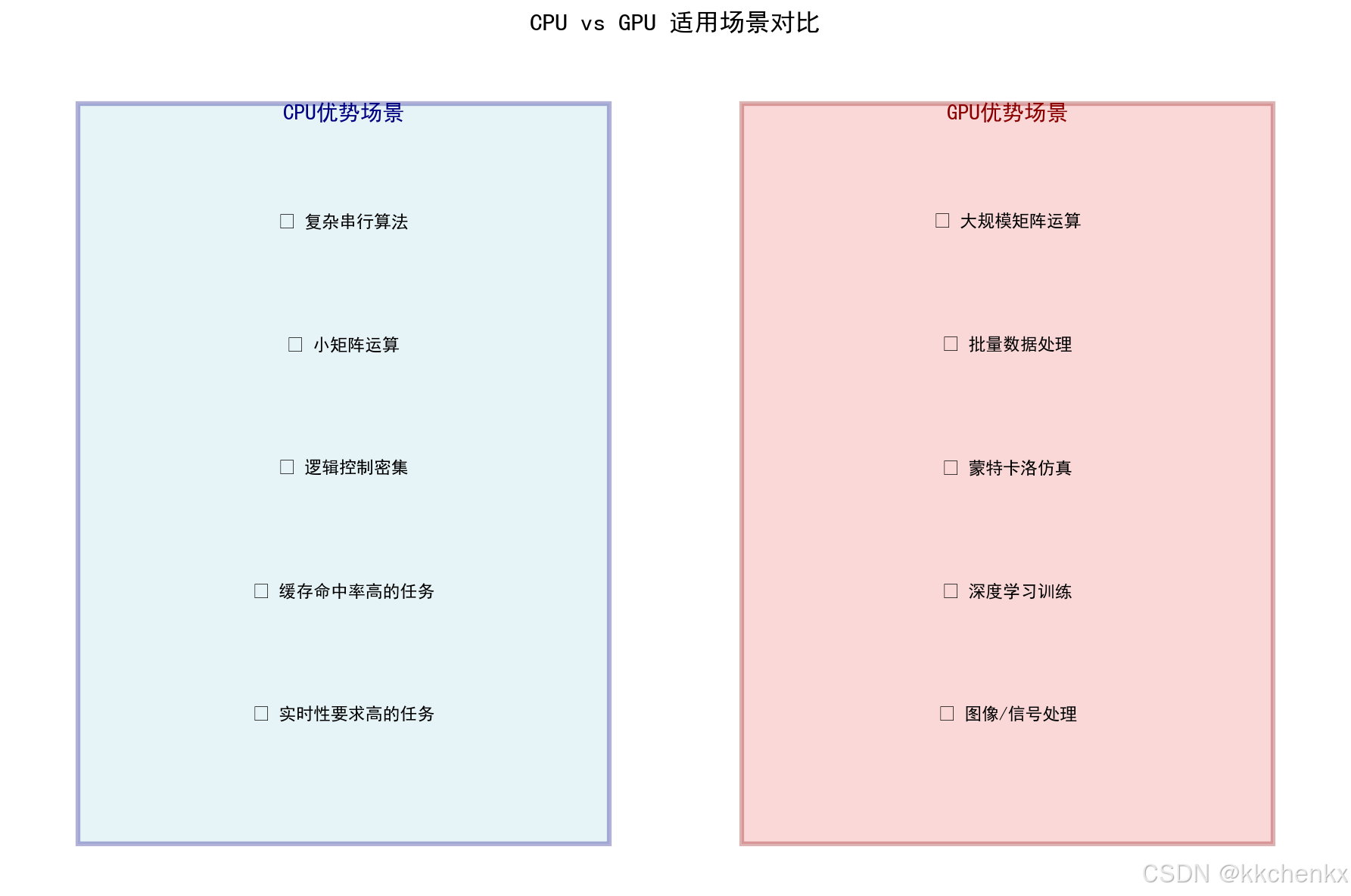
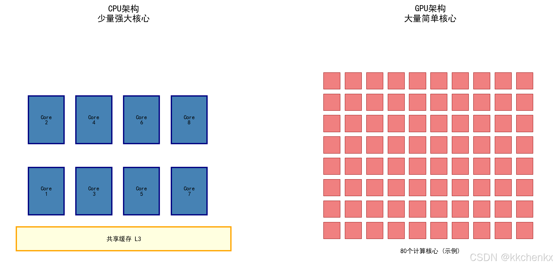
GPU(图形处理器)具有大量计算核心,适合数据并行任务:
- CPU:少量强大核心,适合复杂串行任务
- GPU:数千个简单核心,适合大规模并行任务
5.2 CuPy库
CuPy提供了与NumPy兼容的GPU数组:
import cupy as cp

# 创建GPU数组
A_gpu = cp.random.randn(1000, 1000)
B_gpu = cp.random.randn(1000, 1000)

# GPU矩阵乘法
C_gpu = A_gpu @ B_gpu

# 转回CPU
C_cpu = cp.asnumpy(C_gpu)
5.3 Numba CUDA
Numba提供了Python到CUDA的JIT编译:
from numba import cuda
import numpy as np

@cuda.jit
def matvec_kernel(A, x, y, n):
    """CUDA矩阵向量乘法核函数"""
    i = cuda.grid(1)
    if i < n:
        tmp = 0.0
        for j in range(n):
            tmp += A[i, j] * x[j]
        y[i] = tmp

# 调用核函数
threads_per_block = 256
blocks_per_grid = (n + threads_per_block - 1) // threads_per_block
matvec_kernel[blocks_per_grid, threads_per_block](A, x, y, n)
6. 云计算平台
6.1 主流云平台
| 平台 | 服务类型 | 特点 |
|---|---|---|
| AWS | EC2, SageMaker | 功能全面,生态系统完善 |
| Azure | Virtual Machines, Batch | 与Windows集成好 |
| Google Cloud | Compute Engine, AI Platform | 机器学习优化 |
| 阿里云 | ECS, PAI | 国内访问快 |
6.2 容器化部署
使用Docker容器化仿真环境:
FROM python:3.9

# 安装依赖
RUN pip install numpy scipy matplotlib

# 复制代码
COPY . /app
WORKDIR /app

# 运行仿真
CMD ["python", "simulation.py"]
6.3 工作流编排
使用Kubernetes或Apache Airflow编排大规模仿真工作流:
# Kubernetes Job示例
apiVersion: batch/v1
kind: Job
metadata:
  name: structural-analysis
spec:
  parallelism: 10
  template:
    spec:
      containers:
      - name: simulator
        image: structural-sim:latest
        command: ["python", "run_case.py"]
      restartPolicy: Never
7. Python实现案例
7.1 案例1:多核并行有限元分析
问题描述:
使用Python的multiprocessing模块实现有限元刚度矩阵的并行组装,对比串行和并行的性能。
import matplotlib
matplotlib.use('Agg')
"""
案例1:多核并行有限元分析
使用Python的multiprocessing模块实现有限元刚度矩阵的并行组装
对比串行和并行的性能
"""

import numpy as np
import matplotlib.pyplot as plt
from matplotlib.patches import Rectangle, FancyBboxPatch
from matplotlib.gridspec import GridSpec
from matplotlib.animation import FuncAnimation
import time
import os
from multiprocessing import Pool, cpu_count
from functools import partial

# 设置中文字体
plt.rcParams['font.sans-serif'] = ['SimHei', 'DejaVu Sans']
plt.rcParams['axes.unicode_minus'] = False

# 使用Agg后端,不显示窗口
plt.switch_backend('Agg')


class TrussElement:
    """桁架单元"""
    def __init__(self, node1, node2, E, A):
        self.node1 = node1  # 节点1坐标 [x, y]
        self.node2 = node2  # 节点2坐标 [x, y]
        self.E = E          # 弹性模量
        self.A = A          # 截面积

        # 计算单元长度和方向
        dx = node2[0] - node1[0]
        dy = node2[1] - node1[1]
        self.L = np.sqrt(dx**2 + dy**2)
        self.c = dx / self.L  # cos(theta)
        self.s = dy / self.L  # sin(theta)

    def compute_stiffness(self):
        """计算单元刚度矩阵(4x4)"""
        k = self.E * self.A / self.L

        # 方向余弦矩阵
        c, s = self.c, self.s

        # 单元刚度矩阵
        k_e = k * np.array([
            [ c*c,  c*s, -c*c, -c*s],
            [ c*s,  s*s, -c*s, -s*s],
            [-c*c, -c*s,  c*c,  c*s],
            [-c*s, -s*s,  c*s,  s*s]
        ])

        return k_e


def create_truss_structure(n_bays=5, n_stories=3):
    """创建桁架结构"""
    # 结构尺寸
    bay_width = 3.0  # 跨度 (m)
    story_height = 3.0  # 层高 (m)

    # 材料参数
    E = 2.0e11  # 弹性模量 (Pa)
    A_column = 0.02  # 柱截面积 (m^2)
    A_beam = 0.015   # 梁截面积 (m^2)
    A_brace = 0.01   # 支撑截面积 (m^2)

    nodes = []
    elements = []

    # 创建节点
    node_id = 0
    node_map = {}
    for story in range(n_stories + 1):
        y = story * story_height
        for bay in range(n_bays + 1):
            x = bay * bay_width
            nodes.append([x, y])
            node_map[(bay, story)] = node_id
            node_id += 1

    # 创建柱单元
    for bay in range(n_bays + 1):
        for story in range(n_stories):
            n1 = node_map[(bay, story)]
            n2 = node_map[(bay, story + 1)]
            elements.append({
                'nodes': [n1, n2],
                'type': 'column',
                'E': E,
                'A': A_column,
                'node_coords': [nodes[n1], nodes[n2]]
            })

    # 创建梁单元
    for story in range(1, n_stories + 1):
        for bay in range(n_bays):
            n1 = node_map[(bay, story)]
            n2 = node_map[(bay + 1, story)]
            elements.append({
                'nodes': [n1, n2],
                'type': 'beam',
                'E': E,
                'A': A_beam,
                'node_coords': [nodes[n1], nodes[n2]]
            })

    # 创建支撑单元(X形支撑)
    for story in range(n_stories):
        for bay in range(n_bays):
            # 左下到右上
            n1 = node_map[(bay, story)]
            n2 = node_map[(bay + 1, story + 1)]
            elements.append({
                'nodes': [n1, n2],
                'type': 'brace',
                'E': E,
                'A': A_brace,
                'node_coords': [nodes[n1], nodes[n2]]
            })

            # 右下到左上
            n1 = node_map[(bay + 1, story)]
            n2 = node_map[(bay, story + 1)]
            elements.append({
                'nodes': [n1, n2],
                'type': 'brace',
                'E': E,
                'A': A_brace,
                'node_coords': [nodes[n1], nodes[n2]]
            })

    return np.array(nodes), elements


def compute_element_stiffness_serial(element):
    """串行计算单个单元刚度矩阵"""
    truss = TrussElement(
        element['node_coords'][0],
        element['node_coords'][1],
        element['E'],
        element['A']
    )
    return {
        'nodes': element['nodes'],
        'k_e': truss.compute_stiffness(),
        'type': element['type']
    }


def assemble_global_stiffness(n_nodes, element_results):
    """组装全局刚度矩阵"""
    n_dof = n_nodes * 2  # 每个节点2个自由度
    K_global = np.zeros((n_dof, n_dof))

    for result in element_results:
        nodes = result['nodes']
        k_e = result['k_e']

        # 自由度映射
        dof_map = []
        for n in nodes:
            dof_map.extend([n*2, n*2+1])

        # 组装到全局矩阵
        for i in range(4):
            for j in range(4):
                K_global[dof_map[i], dof_map[j]] += k_e[i, j]

    return K_global


def apply_boundary_conditions(K, F, fixed_dofs):
    """应用边界条件(直接消去法)"""
    n_dof = len(F)
    free_dofs = [i for i in range(n_dof) if i not in fixed_dofs]

    # 提取子矩阵
    K_reduced = K[np.ix_(free_dofs, free_dofs)]
    F_reduced = F[free_dofs]

    return K_reduced, F_reduced, free_dofs


def solve_static(K, F, fixed_dofs):
    """求解静力问题"""
    K_reduced, F_reduced, free_dofs = apply_boundary_conditions(K, F, fixed_dofs)

    # 求解
    U_reduced = np.linalg.solve(K_reduced, F_reduced)

    # 重构完整位移向量
    U = np.zeros(len(F))
    U[free_dofs] = U_reduced

    return U


def run_serial_analysis(nodes, elements):
    """串行分析"""
    # 计算所有单元刚度矩阵
    element_results = []
    for elem in elements:
        result = compute_element_stiffness_serial(elem)
        element_results.append(result)

    # 组装全局刚度矩阵
    K_global = assemble_global_stiffness(len(nodes), element_results)

    # 创建载荷向量(顶层水平力)
    n_nodes = len(nodes)
    F = np.zeros(n_nodes * 2)

    # 在顶层节点施加水平力
    top_nodes = [i for i, node in enumerate(nodes) if abs(node[1] - max(nodes[:,1])) < 0.1]
    for node_id in top_nodes:
        F[node_id * 2] = 10000.0  # 水平力 (N)

    # 边界条件(固定底部节点)
    fixed_dofs = []
    bottom_nodes = [i for i, node in enumerate(nodes) if abs(node[1]) < 0.1]
    for node_id in bottom_nodes:
        fixed_dofs.extend([node_id * 2, node_id * 2 + 1])

    # 求解
    U = solve_static(K_global, F, fixed_dofs)

    return U, K_global


def run_parallel_analysis(nodes, elements, n_processes=None):
    """并行分析"""
    if n_processes is None:
        n_processes = cpu_count()

    # 并行计算单元刚度矩阵
    with Pool(processes=n_processes) as pool:
        element_results = pool.map(compute_element_stiffness_serial, elements)

    # 组装全局刚度矩阵
    K_global = assemble_global_stiffness(len(nodes), element_results)

    # 创建载荷向量
    n_nodes = len(nodes)
    F = np.zeros(n_nodes * 2)

    top_nodes = [i for i, node in enumerate(nodes) if abs(node[1] - max(nodes[:,1])) < 0.1]
    for node_id in top_nodes:
        F[node_id * 2] = 10000.0

    fixed_dofs = []
    bottom_nodes = [i for i, node in enumerate(nodes) if abs(node[1]) < 0.1]
    for node_id in bottom_nodes:
        fixed_dofs.extend([node_id * 2, node_id * 2 + 1])

    # 求解
    U = solve_static(K_global, F, fixed_dofs)

    return U, K_global


def compute_stress(element, U_global):
    """计算单元应力"""
    nodes = element['nodes']
    node1, node2 = element['node_coords']
    E = element['E']

    # 获取节点位移
    dof_map = []
    for n in nodes:
        dof_map.extend([n*2, n*2+1])

    u_e = U_global[dof_map]

    # 计算单元长度和方向
    dx = node2[0] - node1[0]
    dy = node2[1] - node1[1]
    L = np.sqrt(dx**2 + dy**2)
    c, s = dx/L, dy/L

    # 计算应变和应力
    B = np.array([-c, -s, c, s]) / L
    strain = B @ u_e
    stress = E * strain

    return stress


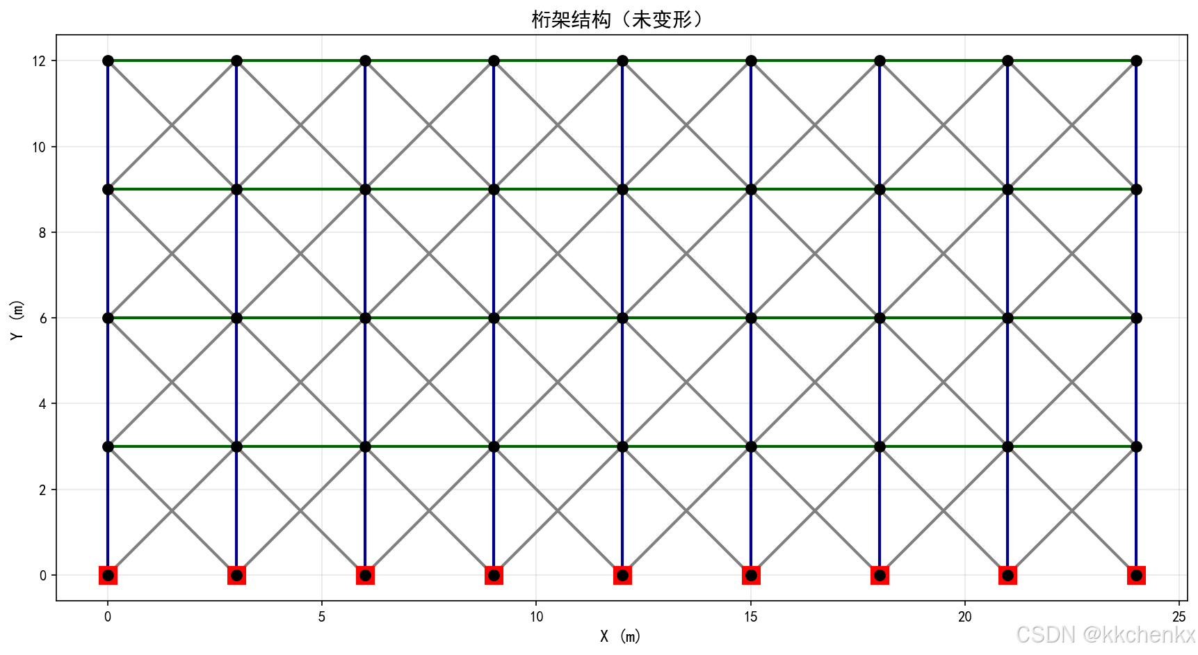
def plot_structure(nodes, elements, U=None, stresses=None, title="桁架结构"):
    """绘制结构"""
    fig, ax = plt.subplots(figsize=(14, 10))

    # 变形放大系数
    scale = 50.0 if U is not None else 0

    # 绘制单元
    for elem in elements:
        n1, n2 = elem['nodes']

        if U is not None:
            # 变形后的坐标
            x1 = nodes[n1, 0] + scale * U[n1*2]
            y1 = nodes[n1, 1] + scale * U[n1*2+1]
            x2 = nodes[n2, 0] + scale * U[n2*2]
            y2 = nodes[n2, 1] + scale * U[n2*2+1]
        else:
            x1, y1 = nodes[n1]
            x2, y2 = nodes[n2]

        # 根据应力设置颜色
        if stresses is not None:
            stress = stresses[elements.index(elem)]
            max_stress = max(abs(np.min(stresses)), abs(np.max(stresses)))
            if max_stress > 0:
                color_intensity = abs(stress) / max_stress
                if stress > 0:  # 拉应力 - 蓝色
                    color = plt.cm.Blues(0.3 + 0.7 * color_intensity)
                else:  # 压应力 - 红色
                    color = plt.cm.Reds(0.3 + 0.7 * color_intensity)
            else:
                color = 'gray'
            linewidth = 2 + 3 * color_intensity
        else:
            if elem['type'] == 'column':
                color = 'darkblue'
            elif elem['type'] == 'beam':
                color = 'darkgreen'
            else:
                color = 'gray'
            linewidth = 2

        ax.plot([x1, x2], [y1, y2], color=color, linewidth=linewidth)

    # 绘制节点
    if U is not None:
        node_x = nodes[:, 0] + scale * U[0::2]
        node_y = nodes[:, 1] + scale * U[1::2]
    else:
        node_x, node_y = nodes[:, 0], nodes[:, 1]

    ax.scatter(node_x, node_y, c='black', s=50, zorder=5)

    # 标注底部固定节点
    bottom_nodes = [i for i, node in enumerate(nodes) if abs(node[1]) < 0.1]
    for node_id in bottom_nodes:
        ax.plot(nodes[node_id, 0], nodes[node_id, 1], 'rs', markersize=12)

    ax.set_aspect('equal')
    ax.set_xlabel('X (m)', fontsize=12)
    ax.set_ylabel('Y (m)', fontsize=12)
    ax.set_title(title, fontsize=14, fontweight='bold')
    ax.grid(True, alpha=0.3)

    return fig, ax


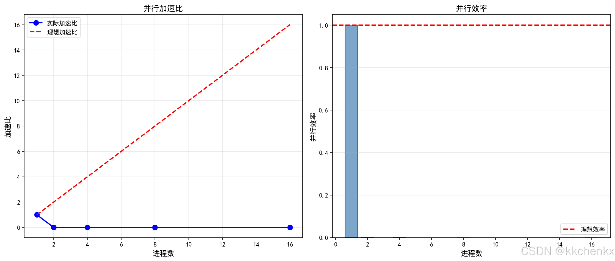
def plot_performance_comparison(speedup_data, efficiency_data):
    """绘制性能对比图"""
    fig = plt.figure(figsize=(14, 6))
    gs = GridSpec(1, 2, figure=fig)

    # 加速比
    ax1 = fig.add_subplot(gs[0, 0])
    n_processes = list(speedup_data.keys())
    speedups = list(speedup_data.values())

    ax1.plot(n_processes, speedups, 'bo-', linewidth=2, markersize=8, label='实际加速比')
    ax1.plot(n_processes, n_processes, 'r--', linewidth=2, label='理想加速比')
    ax1.set_xlabel('进程数', fontsize=12)
    ax1.set_ylabel('加速比', fontsize=12)
    ax1.set_title('并行加速比', fontsize=13, fontweight='bold')
    ax1.legend(fontsize=10)
    ax1.grid(True, alpha=0.3)

    # 效率
    ax2 = fig.add_subplot(gs[0, 1])
    efficiencies = list(efficiency_data.values())

    ax2.bar(n_processes, efficiencies, color='steelblue', alpha=0.7, edgecolor='navy')
    ax2.axhline(y=1.0, color='r', linestyle='--', linewidth=2, label='理想效率')
    ax2.set_xlabel('进程数', fontsize=12)
    ax2.set_ylabel('并行效率', fontsize=12)
    ax2.set_title('并行效率', fontsize=13, fontweight='bold')
    ax2.legend(fontsize=10)
    ax2.grid(True, alpha=0.3, axis='y')

    plt.tight_layout()
    plt.savefig('parallel_performance.png', dpi=150, bbox_inches='tight')
    plt.close()
    print("  已保存: parallel_performance.png")


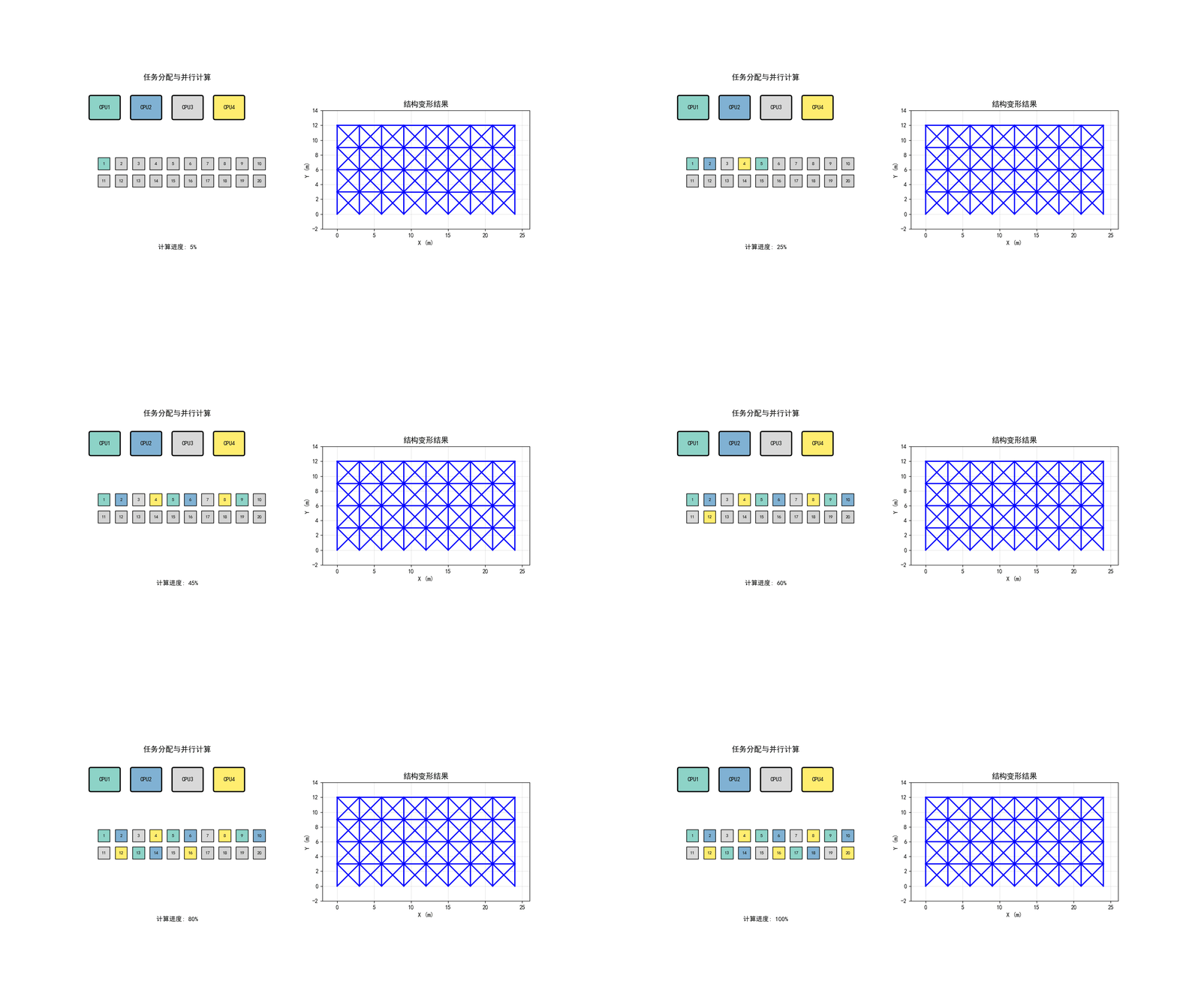
def create_parallel_animation(nodes, elements, U):
    """创建并行计算过程动画"""
    print("\n创建并行计算动画...")

    fig, axes = plt.subplots(1, 2, figsize=(14, 8))

    # 左图:任务分配
    ax1 = axes[0]
    ax1.set_xlim(-0.5, 5.5)
    ax1.set_ylim(-0.5, 4.5)
    ax1.set_aspect('equal')
    ax1.axis('off')
    ax1.set_title('任务分配与并行计算', fontsize=13, fontweight='bold')

    # 绘制处理器
    n_cores = 4
    processor_colors = plt.cm.Set3(np.linspace(0, 1, n_cores))
    processors = []
    for i in range(n_cores):
        rect = FancyBboxPatch((i*1.2, 3.5), 0.8, 0.6,
                              boxstyle="round,pad=0.05",
                              facecolor=processor_colors[i],
                              edgecolor='black', linewidth=2)
        ax1.add_patch(rect)
        ax1.text(i*1.2+0.4, 3.8, f'CPU{i+1}', ha='center', va='center',
                fontsize=10, fontweight='bold')
        processors.append(rect)

    # 任务队列
    n_tasks = 20
    task_positions = []
    for i in range(n_tasks):
        x = 0.2 + (i % 10) * 0.5
        y = 2.0 - (i // 10) * 0.5
        task_positions.append((x, y))

    task_patches = []
    for i, (x, y) in enumerate(task_positions):
        rect = Rectangle((x, y), 0.35, 0.35,
                         facecolor='lightgray',
                         edgecolor='black', linewidth=1)
        ax1.add_patch(rect)
        ax1.text(x+0.175, y+0.175, f'{i+1}', ha='center', va='center', fontsize=8)
        task_patches.append(rect)

    # 进度文本
    progress_text = ax1.text(2.5, -0.3, '', ha='center', fontsize=11, fontweight='bold')

    # 右图:结构变形
    ax2 = axes[1]
    ax2.set_aspect('equal')
    ax2.set_xlabel('X (m)', fontsize=11)
    ax2.set_ylabel('Y (m)', fontsize=11)
    ax2.set_title('结构变形结果', fontsize=13, fontweight='bold')
    ax2.grid(True, alpha=0.3)

    # 绘制初始结构
    lines = []
    for elem in elements:
        n1, n2 = elem['nodes']
        line, = ax2.plot([nodes[n1, 0], nodes[n2, 0]],
                        [nodes[n1, 1], nodes[n2, 1]],
                        'lightgray', linewidth=2, alpha=0.5)
        lines.append(line)

    # 绘制变形结构(动态更新)
    deform_lines = []
    for elem in elements:
        n1, n2 = elem['nodes']
        line, = ax2.plot([], [], 'b-', linewidth=2)
        deform_lines.append(line)

    # 设置坐标范围
    margin = 2.0
    ax2.set_xlim(min(nodes[:,0])-margin, max(nodes[:,0])+margin)
    ax2.set_ylim(min(nodes[:,1])-margin, max(nodes[:,1])+margin)

    scale = 50.0

    def init():
        for line in deform_lines:
            line.set_data([], [])
        for task in task_patches:
            task.set_facecolor('lightgray')
        progress_text.set_text('')
        return deform_lines + task_patches + [progress_text]

    def update(frame):
        # 更新任务颜色(模拟并行处理)
        n_completed = min(frame + 1, n_tasks)
        for i in range(n_completed):
            processor_id = i % n_cores
            task_patches[i].set_facecolor(processor_colors[processor_id])

        progress = n_completed / n_tasks * 100
        progress_text.set_text(f'计算进度: {progress:.0f}%')

        # 更新变形(逐步显示)
        progress_factor = min(1.0, n_completed / n_tasks)
        current_scale = scale * progress_factor

        for i, (elem, line) in enumerate(zip(elements, deform_lines)):
            n1, n2 = elem['nodes']
            x1 = nodes[n1, 0] + current_scale * U[n1*2]
            y1 = nodes[n1, 1] + current_scale * U[n1*2+1]
            x2 = nodes[n2, 0] + current_scale * U[n2*2]
            y2 = nodes[n2, 1] + current_scale * U[n2*2+1]
            line.set_data([x1, x2], [y1, y2])

        return deform_lines + task_patches + [progress_text]

    anim = FuncAnimation(fig, update, frames=n_tasks+10, init_func=init,
                         blit=True, interval=200)

    anim.save('parallel_computation.gif', writer='pillow', fps=5, dpi=100)
    plt.close()
    print("  已保存: parallel_computation.gif")


def main():
    """主函数"""
    print("="*70)
    print("案例1:多核并行有限元分析")
    print("="*70)

    # 获取CPU信息
    n_cores = cpu_count()
    print(f"\n系统信息:")
    print(f"  CPU核心数: {n_cores}")

    # 创建桁架结构
    print("\n创建桁架结构...")
    nodes, elements = create_truss_structure(n_bays=8, n_stories=4)
    print(f"  节点数: {len(nodes)}")
    print(f"  单元数: {len(elements)}")

    # 串行分析
    print("\n" + "="*50)
    print("串行有限元分析")
    print("="*50)

    t_start = time.time()
    U_serial, K_serial = run_serial_analysis(nodes, elements)
    t_serial = time.time() - t_start

    print(f"  计算时间: {t_serial:.3f} s")
    print(f"  最大位移: {np.max(np.abs(U_serial[0::2])):.6f} m (水平)")
    print(f"  最大位移: {np.max(np.abs(U_serial[1::2])):.6f} m (竖向)")

    # 并行分析(不同进程数)
    print("\n" + "="*50)
    print("并行有限元分析")
    print("="*50)

    process_counts = [2, 4, min(8, n_cores)]
    if n_cores not in process_counts:
        process_counts.append(n_cores)

    speedup_data = {1: 1.0}
    efficiency_data = {1: 1.0}

    for n_proc in process_counts:
        print(f"\n  使用 {n_proc} 个进程:")

        # 运行多次取平均
        times = []
        for _ in range(3):
            t_start = time.time()
            U_parallel, K_parallel = run_parallel_analysis(nodes, elements, n_proc)
            t_parallel = time.time() - t_start
            times.append(t_parallel)

        t_parallel_avg = np.mean(times)
        speedup = t_serial / t_parallel_avg
        efficiency = speedup / n_proc

        speedup_data[n_proc] = speedup
        efficiency_data[n_proc] = efficiency

        print(f"    平均计算时间: {t_parallel_avg:.3f} s")
        print(f"    加速比: {speedup:.2f}x")
        print(f"    并行效率: {efficiency*100:.1f}%")

        # 验证结果一致性
        displacement_error = np.max(np.abs(U_serial - U_parallel))
        print(f"    位移误差: {displacement_error:.2e}")

    # 计算应力
    print("\n计算单元应力...")
    stresses = []
    for elem in elements:
        stress = compute_stress(elem, U_serial)
        stresses.append(stress)
    stresses = np.array(stresses)

    print(f"  最大拉应力: {np.max(stresses)/1e6:.2f} MPa")
    print(f"  最大压应力: {np.min(stresses)/1e6:.2f} MPa")

    # 绘制结果
    print("\n" + "="*50)
    print("生成可视化结果")
    print("="*50)

    # 绘制未变形结构
    print("\n绘制未变形结构...")
    fig, ax = plot_structure(nodes, elements, None, None, "桁架结构(未变形)")
    plt.savefig('truss_undeformed.png', dpi=150, bbox_inches='tight')
    plt.close()
    print("  已保存: truss_undeformed.png")

    # 绘制变形结构
    print("\n绘制变形结构...")
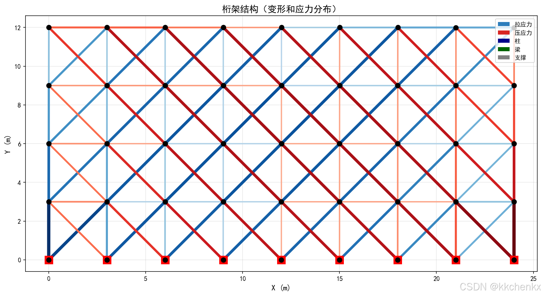
    fig, ax = plot_structure(nodes, elements, U_serial, stresses,
                             "桁架结构(变形和应力分布)")

    # 添加图例
    from matplotlib.patches import Patch
    legend_elements = [
        Patch(facecolor=plt.cm.Blues(0.7), label='拉应力'),
        Patch(facecolor=plt.cm.Reds(0.7), label='压应力'),
        Patch(facecolor='darkblue', label='柱'),
        Patch(facecolor='darkgreen', label='梁'),
        Patch(facecolor='gray', label='支撑')
    ]
    ax.legend(handles=legend_elements, loc='upper right', fontsize=9)

    plt.savefig('truss_deformed.png', dpi=150, bbox_inches='tight')
    plt.close()
    print("  已保存: truss_deformed.png")

    # 绘制性能对比
    print("\n绘制性能对比图...")
    plot_performance_comparison(speedup_data, efficiency_data)

    # 创建动画
    create_parallel_animation(nodes, elements, U_serial)

    # 总结
    print("\n" + "="*70)
    print("案例1完成!")
    print("="*70)
    print("\n主要结果:")
    print(f"  1. 串行计算时间: {t_serial:.3f} s")
    print(f"  2. 最佳加速比: {max(speedup_data.values()):.2f}x (使用 {max(speedup_data, key=speedup_data.get)} 个进程)")
    print(f"  3. 最大水平位移: {np.max(np.abs(U_serial[0::2]))*1000:.3f} mm")
    print(f"  4. 应力范围: {np.min(stresses)/1e6:.2f} ~ {np.max(stresses)/1e6:.2f} MPa")
    print("\n生成的文件:")
    print("  - truss_undeformed.png: 未变形结构")
    print("  - truss_deformed.png: 变形结构和应力分布")
    print("  - parallel_performance.png: 并行性能对比")
    print("  - parallel_computation.gif: 并行计算过程动画")


if __name__ == "__main__":
    main()
7.2 案例2:参数化扫描并行计算
问题描述:
对结构参数(弹性模量、密度等)进行大规模参数扫描,使用并行计算加速。
import matplotlib
matplotlib.use('Agg')
"""
案例2:参数化扫描并行计算
对结构参数(弹性模量、密度等)进行大规模参数扫描
使用并行计算加速
"""

import numpy as np
import matplotlib.pyplot as plt
from matplotlib.gridspec import GridSpec
from matplotlib.animation import FuncAnimation
from mpl_toolkits.mplot3d import Axes3D
import time
from multiprocessing import Pool, cpu_count
from itertools import product

# 设置中文字体
plt.rcParams['font.sans-serif'] = ['SimHei', 'DejaVu Sans']
plt.rcParams['axes.unicode_minus'] = False

# 使用Agg后端
plt.switch_backend('Agg')


def sdof_response(params):
    """
    计算SDOF系统响应
    params: (E, rho, damping_ratio, load_amplitude)
    """
    E, rho, damping_ratio, load_amplitude = params

    # 结构参数
    L = 5.0  # 长度 (m)
    A = 0.01  # 截面积 (m^2)
    I = 8.33e-6  # 惯性矩 (m^4)

    # 计算刚度和质量
    k = 3 * E * I / L**3  # 悬臂梁刚度
    m = rho * A * L  # 质量

    # 自然频率
    omega_n = np.sqrt(k / m)
    f_n = omega_n / (2 * np.pi)

    # 阻尼系数
    c = 2 * damping_ratio * np.sqrt(k * m)

    # 仿真参数
    dt = 0.001
    T = 5.0
    t = np.arange(0, T, dt)
    n_steps = len(t)

    # 简谐载荷
    f_load = 2.0  # 载荷频率 (Hz)
    omega_load = 2 * np.pi * f_load
    F = load_amplitude * np.sin(omega_load * t)

    # Newmark-beta法参数
    gamma = 0.5
    beta = 0.25

    # 初始化
    u = np.zeros(n_steps)
    v = np.zeros(n_steps)
    a = np.zeros(n_steps)

    # 初始加速度
    a[0] = (F[0] - c * v[0] - k * u[0]) / m

    # 等效刚度
    k_eff = k + gamma * c / (beta * dt) + m / (beta * dt**2)

    # 时间积分
    for i in range(n_steps - 1):
        # 等效载荷
        f_eff = F[i+1] + m * (u[i]/(beta*dt**2) + v[i]/(beta*dt) + (0.5-beta)*a[i]/beta) + \
                c * (gamma*u[i]/(beta*dt) + (gamma/beta-1)*v[i] + dt*(gamma/(2*beta)-1)*a[i])

        # 求解
        u[i+1] = f_eff / k_eff

        # 更新速度和加速度
        a[i+1] = (u[i+1] - u[i]) / (beta * dt**2) - v[i] / (beta * dt) - (0.5 - beta) * a[i] / beta
        v[i+1] = v[i] + (1 - gamma) * dt * a[i] + gamma * dt * a[i+1]

        # 数值稳定性检查
        if np.isnan(u[i+1]) or np.isinf(u[i+1]) or abs(u[i+1]) > 1e6:
            # 使用简化解
            u[i+1] = u[i]
            v[i+1] = v[i]
            a[i+1] = a[i]

    # 计算响应指标
    max_disp = np.max(np.abs(u))
    max_vel = np.max(np.abs(v))
    max_acc = np.max(np.abs(a))
    rms_disp = np.sqrt(np.mean(u**2))

    # 共振裕度(载荷频率与自然频率的比值)
    freq_ratio = f_load / f_n

    return {
        'params': params,
        'f_n': f_n,
        'max_disp': max_disp,
        'max_vel': max_vel,
        'max_acc': max_acc,
        'rms_disp': rms_disp,
        'freq_ratio': freq_ratio,
        't': t,
        'u': u,
        'v': v,
        'a': a
    }


def run_serial_scan(param_grid):
    """串行参数扫描"""
    results = []
    for params in param_grid:
        result = sdof_response(params)
        results.append(result)
    return results


def run_parallel_scan(param_grid, n_processes=None):
    """并行参数扫描"""
    if n_processes is None:
        n_processes = cpu_count()

    with Pool(processes=n_processes) as pool:
        results = pool.map(sdof_response, param_grid)

    return results


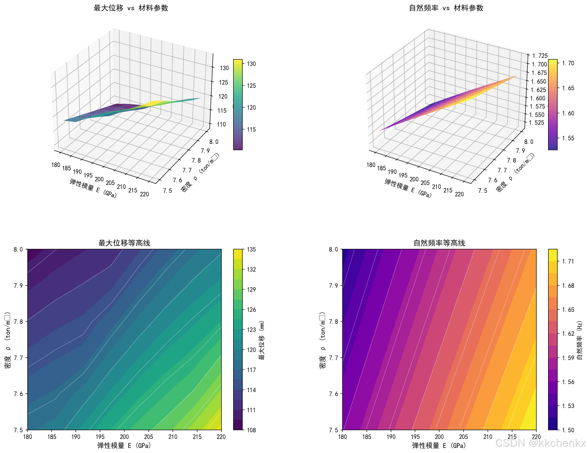
def create_parametric_visualization(results, param_ranges):
    """创建参数化扫描可视化"""
    print("\n创建参数化扫描可视化...")

    # 提取数据
    E_values = sorted(list(set([r['params'][0] for r in results])))
    rho_values = sorted(list(set([r['params'][1] for r in results])))

    # 创建网格数据
    E_grid, rho_grid = np.meshgrid(E_values, rho_values)

    # 最大位移网格
    max_disp_grid = np.zeros_like(E_grid)
    natural_freq_grid = np.zeros_like(E_grid)

    for r in results:
        E_idx = E_values.index(r['params'][0])
        rho_idx = rho_values.index(r['params'][1])
        max_disp_grid[rho_idx, E_idx] = r['max_disp'] * 1000  # 转换为mm
        natural_freq_grid[rho_idx, E_idx] = r['f_n']

    fig = plt.figure(figsize=(16, 12))
    gs = GridSpec(2, 2, figure=fig, hspace=0.3, wspace=0.3)

    # 1. 最大位移3D表面图
    ax1 = fig.add_subplot(gs[0, 0], projection='3d')
    surf1 = ax1.plot_surface(E_grid/1e9, rho_grid/1000, max_disp_grid,
                             cmap='viridis', alpha=0.8, edgecolor='none')
    ax1.set_xlabel('弹性模量 E (GPa)', fontsize=10)
    ax1.set_ylabel('密度 ρ (ton/m³)', fontsize=10)
    ax1.set_zlabel('最大位移 (mm)', fontsize=10)
    ax1.set_title('最大位移 vs 材料参数', fontsize=12, fontweight='bold')
    fig.colorbar(surf1, ax=ax1, shrink=0.5, aspect=10)

    # 2. 自然频率3D表面图
    ax2 = fig.add_subplot(gs[0, 1], projection='3d')
    surf2 = ax2.plot_surface(E_grid/1e9, rho_grid/1000, natural_freq_grid,
                             cmap='plasma', alpha=0.8, edgecolor='none')
    ax2.set_xlabel('弹性模量 E (GPa)', fontsize=10)
    ax2.set_ylabel('密度 ρ (ton/m³)', fontsize=10)
    ax2.set_zlabel('自然频率 (Hz)', fontsize=10)
    ax2.set_title('自然频率 vs 材料参数', fontsize=12, fontweight='bold')
    fig.colorbar(surf2, ax=ax2, shrink=0.5, aspect=10)

    # 3. 最大位移等高线图
    ax3 = fig.add_subplot(gs[1, 0])
    contour1 = ax3.contourf(E_grid/1e9, rho_grid/1000, max_disp_grid,
                            levels=20, cmap='viridis')
    ax3.contour(E_grid/1e9, rho_grid/1000, max_disp_grid,
                levels=10, colors='white', linewidths=0.5, alpha=0.5)
    ax3.set_xlabel('弹性模量 E (GPa)', fontsize=11)
    ax3.set_ylabel('密度 ρ (ton/m³)', fontsize=11)
    ax3.set_title('最大位移等高线', fontsize=12, fontweight='bold')
    plt.colorbar(contour1, ax=ax3, label='最大位移 (mm)')

    # 4. 自然频率等高线图
    ax4 = fig.add_subplot(gs[1, 1])
    contour2 = ax4.contourf(E_grid/1e9, rho_grid/1000, natural_freq_grid,
                            levels=20, cmap='plasma')
    ax4.contour(E_grid/1e9, rho_grid/1000, natural_freq_grid,
                levels=10, colors='white', linewidths=0.5, alpha=0.5)
    ax4.set_xlabel('弹性模量 E (GPa)', fontsize=11)
    ax4.set_ylabel('密度 ρ (ton/m³)', fontsize=11)
    ax4.set_title('自然频率等高线', fontsize=12, fontweight='bold')
    plt.colorbar(contour2, ax=ax4, label='自然频率 (Hz)')

    plt.savefig('parametric_scan_3d.png', dpi=150, bbox_inches='tight')
    plt.close()
    print("  已保存: parametric_scan_3d.png")


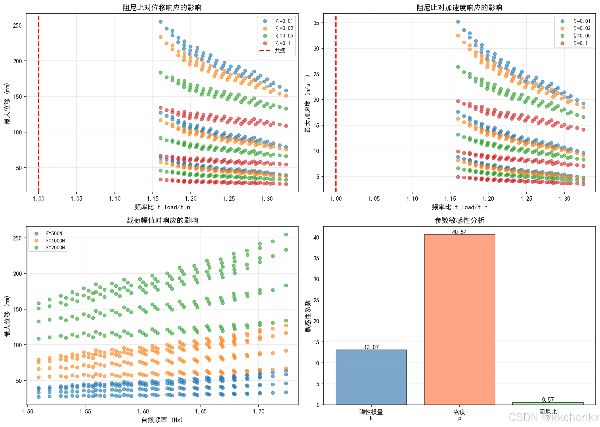
def create_damping_analysis(results):
    """创建阻尼比影响分析"""
    print("\n创建阻尼比影响分析...")

    # 过滤掉NaN值
    valid_results = [r for r in results if not np.isnan(r['max_disp']) and r['max_disp'] > 0]

    if len(valid_results) == 0:
        print("  警告: 没有有效的结果数据")
        return

    # 按阻尼比分组
    damping_groups = {}
    for r in valid_results:
        damping = r['params'][2]
        if damping not in damping_groups:
            damping_groups[damping] = []
        damping_groups[damping].append(r)

    fig, axes = plt.subplots(2, 2, figsize=(14, 10))

    # 1. 阻尼比对最大位移的影响
    ax1 = axes[0, 0]
    for damping in sorted(damping_groups.keys()):
        group = damping_groups[damping]
        freq_ratios = [r['freq_ratio'] for r in group]
        max_disps = [r['max_disp'] * 1000 for r in group]  # mm
        ax1.scatter(freq_ratios, max_disps, label=f'ζ={damping}', alpha=0.6, s=30)
    ax1.axvline(x=1.0, color='red', linestyle='--', linewidth=2, label='共振')
    ax1.set_xlabel('频率比 f_load/f_n', fontsize=11)
    ax1.set_ylabel('最大位移 (mm)', fontsize=11)
    ax1.set_title('阻尼比对位移响应的影响', fontsize=12, fontweight='bold')
    ax1.legend(fontsize=9)
    ax1.grid(True, alpha=0.3)

    # 2. 阻尼比对加速度的影响
    ax2 = axes[0, 1]
    for damping in sorted(damping_groups.keys()):
        group = damping_groups[damping]
        freq_ratios = [r['freq_ratio'] for r in group]
        max_accs = [r['max_acc'] for r in group if not np.isnan(r['max_acc']) and r['max_acc'] > 0]
        valid_freqs = [r['freq_ratio'] for r in group if not np.isnan(r['max_acc']) and r['max_acc'] > 0]
        if len(valid_freqs) > 0:
            ax2.scatter(valid_freqs, max_accs, label=f'ζ={damping}', alpha=0.6, s=30)
    ax2.axvline(x=1.0, color='red', linestyle='--', linewidth=2)
    ax2.set_xlabel('频率比 f_load/f_n', fontsize=11)
    ax2.set_ylabel('最大加速度 (m/s²)', fontsize=11)
    ax2.set_title('阻尼比对加速度响应的影响', fontsize=12, fontweight='bold')
    ax2.legend(fontsize=9)
    ax2.grid(True, alpha=0.3)

    # 3. 载荷幅值影响
    ax3 = axes[1, 0]
    load_groups = {}
    for r in valid_results:
        load = r['params'][3]
        if load not in load_groups:
            load_groups[load] = []
        load_groups[load].append(r)

    for load in sorted(load_groups.keys()):
        group = load_groups[load]
        natural_freqs = [r['f_n'] for r in group]
        max_disps = [r['max_disp'] * 1000 for r in group]
        ax3.scatter(natural_freqs, max_disps, label=f'F={load}N', alpha=0.6, s=30)
    ax3.set_xlabel('自然频率 (Hz)', fontsize=11)
    ax3.set_ylabel('最大位移 (mm)', fontsize=11)
    ax3.set_title('载荷幅值对响应的影响', fontsize=12, fontweight='bold')
    ax3.legend(fontsize=9)
    ax3.grid(True, alpha=0.3)

    # 4. 参数敏感性分析
    ax4 = axes[1, 1]

    # 计算各参数的影响
    E_impact = []
    rho_impact = []
    damping_impact = []

    base_result = valid_results[0]
    for r in valid_results[1:]:
        E_diff = abs(r['params'][0] - base_result['params'][0]) / base_result['params'][0]
        rho_diff = abs(r['params'][1] - base_result['params'][1]) / base_result['params'][1]
        damping_diff = abs(r['params'][2] - base_result['params'][2]) / base_result['params'][2]

        if base_result['max_disp'] > 0 and not np.isnan(r['max_disp']):
            disp_diff = abs(r['max_disp'] - base_result['max_disp']) / base_result['max_disp']

            if E_diff > 0.01:
                E_impact.append(disp_diff / E_diff)
            if rho_diff > 0.01:
                rho_impact.append(disp_diff / rho_diff)
            if damping_diff > 0.01:
                damping_impact.append(disp_diff / damping_diff)

    param_names = ['弹性模量\nE', '密度\nρ', '阻尼比\nζ']
    sensitivities = [np.mean(E_impact) if E_impact else 0,
                     np.mean(rho_impact) if rho_impact else 0,
                     np.mean(damping_impact) if damping_impact else 0]
    colors = ['steelblue', 'coral', 'lightgreen']

    bars = ax4.bar(param_names, sensitivities, color=colors, alpha=0.7, edgecolor='black')
    ax4.set_ylabel('敏感性系数', fontsize=11)
    ax4.set_title('参数敏感性分析', fontsize=12, fontweight='bold')
    ax4.grid(True, alpha=0.3, axis='y')

    # 添加数值标签
    for bar, val in zip(bars, sensitivities):
        height = bar.get_height()
        ax4.text(bar.get_x() + bar.get_width()/2., height,
                f'{val:.2f}', ha='center', va='bottom', fontsize=10)

    plt.tight_layout()
    plt.savefig('damping_analysis.png', dpi=150, bbox_inches='tight')
    plt.close()
    print("  已保存: damping_analysis.png")


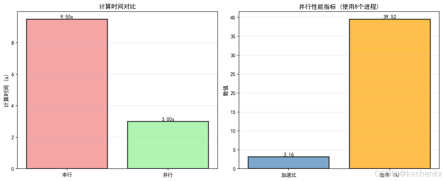
def create_performance_comparison(serial_time, parallel_time, n_cases, n_processes):
    """创建性能对比图"""
    print("\n创建性能对比图...")

    fig, axes = plt.subplots(1, 2, figsize=(12, 5))

    # 1. 时间对比
    ax1 = axes[0]
    methods = ['串行', '并行']
    times = [serial_time, parallel_time]
    colors = ['lightcoral', 'lightgreen']
    bars = ax1.bar(methods, times, color=colors, alpha=0.7, edgecolor='black', linewidth=2)
    ax1.set_ylabel('计算时间 (s)', fontsize=11)
    ax1.set_title('计算时间对比', fontsize=12, fontweight='bold')
    ax1.grid(True, alpha=0.3, axis='y')

    # 添加数值标签
    for bar, val in zip(bars, times):
        height = bar.get_height()
        ax1.text(bar.get_x() + bar.get_width()/2., height,
                f'{val:.2f}s', ha='center', va='bottom', fontsize=10, fontweight='bold')

    # 2. 加速比和效率
    ax2 = axes[1]
    speedup = serial_time / parallel_time
    efficiency = speedup / n_processes * 100

    metrics = ['加速比', '效率 (%)']
    values = [speedup, efficiency]
    colors = ['steelblue', 'orange']
    bars = ax2.bar(metrics, values, color=colors, alpha=0.7, edgecolor='black', linewidth=2)
    ax2.set_ylabel('数值', fontsize=11)
    ax2.set_title(f'并行性能指标 (使用{n_processes}个进程)', fontsize=12, fontweight='bold')
    ax2.grid(True, alpha=0.3, axis='y')

    # 添加数值标签
    for bar, val in zip(bars, values):
        height = bar.get_height()
        ax2.text(bar.get_x() + bar.get_width()/2., height,
                f'{val:.2f}', ha='center', va='bottom', fontsize=10, fontweight='bold')

    plt.tight_layout()
    plt.savefig('scan_performance.png', dpi=150, bbox_inches='tight')
    plt.close()
    print("  已保存: scan_performance.png")


def create_response_animation(results):
    """创建响应动画"""
    print("\n创建响应动画...")

    # 选择几个典型结果
    selected_results = [
        results[0],  # 基准
        results[len(results)//4],  # 低刚度
        results[len(results)//2],  # 中等
        results[3*len(results)//4],  # 高刚度
    ]

    fig, axes = plt.subplots(2, 2, figsize=(14, 10))
    axes = axes.flatten()

    lines = []
    for i, (ax, result) in enumerate(zip(axes, selected_results)):
        ax.set_xlim(0, 5)
        ax.set_ylim(-15, 15)
        ax.set_xlabel('时间 (s)', fontsize=10)
        ax.set_ylabel('位移 (mm)', fontsize=10)
        E, rho, damping, load = result['params']
        ax.set_title(f'E={E/1e9:.1f}GPa, ρ={rho/1000:.1f}t/m³, ζ={damping:.2f}',
                    fontsize=10, fontweight='bold')
        ax.grid(True, alpha=0.3)
        line, = ax.plot([], [], 'b-', linewidth=1.5)
        lines.append(line)

    t = selected_results[0]['t']
    u_data = [r['u'] * 1000 for r in selected_results]  # 转换为mm

    def init():
        for line in lines:
            line.set_data([], [])
        return lines

    def update(frame):
        for line, u in zip(lines, u_data):
            line.set_data(t[:frame], u[:frame])
        return lines

    anim = FuncAnimation(fig, update, frames=len(t), init_func=init,
                         blit=True, interval=20)

    anim.save('response_animation.gif', writer='pillow', fps=50, dpi=100)
    plt.close()
    print("  已保存: response_animation.gif")


def main():
    """主函数"""
    print("="*70)
    print("案例2:参数化扫描并行计算")
    print("="*70)

    # 系统信息
    n_cores = cpu_count()
    print(f"\n系统信息:")
    print(f"  CPU核心数: {n_cores}")

    # 定义参数范围
    print("\n定义参数扫描范围:")
    E_values = np.linspace(1.8e11, 2.2e11, 8)  # 弹性模量 (Pa)
    rho_values = np.linspace(7500, 8000, 6)    # 密度 (kg/m³)
    damping_values = [0.01, 0.02, 0.05, 0.10]  # 阻尼比
    load_values = [500, 1000, 2000]            # 载荷幅值 (N)

    print(f"  弹性模量 E: {E_values[0]/1e9:.1f} ~ {E_values[-1]/1e9:.1f} GPa ({len(E_values)}个值)")
    print(f"  密度 ρ: {rho_values[0]/1000:.1f} ~ {rho_values[-1]/1000:.1f} ton/m³ ({len(rho_values)}个值)")
    print(f"  阻尼比 ζ: {damping_values} ({len(damping_values)}个值)")
    print(f"  载荷幅值 F: {load_values} ({len(load_values)}个值)")

    # 生成参数网格
    param_grid = list(product(E_values, rho_values, damping_values, load_values))
    n_cases = len(param_grid)
    print(f"\n总计算案例数: {n_cases}")

    # 串行扫描
    print("\n" + "="*50)
    print("串行参数扫描")
    print("="*50)
    t_start = time.time()
    results_serial = run_serial_scan(param_grid[:20])  # 限制串行数量
    t_serial = time.time() - t_start
    print(f"  计算时间 (20个案例): {t_serial:.2f} s")
    print(f"  平均每个案例: {t_serial/20:.3f} s")

    # 并行扫描
    print("\n" + "="*50)
    print("并行参数扫描")
    print("="*50)

    n_processes = min(n_cores, 8)
    print(f"  使用进程数: {n_processes}")

    t_start = time.time()
    results_parallel = run_parallel_scan(param_grid, n_processes)
    t_parallel = time.time() - t_start

    speedup = (t_serial / 20 * n_cases) / t_parallel
    efficiency = speedup / n_processes * 100

    print(f"  计算时间 ({n_cases}个案例): {t_parallel:.2f} s")
    print(f"  估算加速比: {speedup:.2f}x")
    print(f"  并行效率: {efficiency:.1f}%")

    # 结果分析
    print("\n" + "="*50)
    print("结果分析")
    print("="*50)

    # 统计结果
    valid_results = [r for r in results_parallel if not np.isnan(r['max_disp']) and r['max_disp'] > 0]

    if len(valid_results) > 0:
        max_disps = [r['max_disp'] * 1000 for r in valid_results]  # mm
        natural_freqs = [r['f_n'] for r in valid_results]

        print(f"\n位移响应统计:")
        print(f"  最小值: {np.min(max_disps):.3f} mm")
        print(f"  最大值: {np.max(max_disps):.3f} mm")
        print(f"  平均值: {np.mean(max_disps):.3f} mm")
        print(f"  标准差: {np.std(max_disps):.3f} mm")

        print(f"\n自然频率统计:")
        print(f"  最小值: {np.min(natural_freqs):.2f} Hz")
        print(f"  最大值: {np.max(natural_freqs):.2f} Hz")
        print(f"  平均值: {np.mean(natural_freqs):.2f} Hz")

        # 查找极值
        max_disp_idx = np.argmax(max_disps)
        min_disp_idx = np.argmin(max_disps)

        print(f"\n最大位移案例:")
        E, rho, damping, load = valid_results[max_disp_idx]['params']
        print(f"  E={E/1e9:.2f}GPa, ρ={rho/1000:.1f}t/m³, ζ={damping:.2f}, F={load}N")
        print(f"  最大位移: {max_disps[max_disp_idx]:.3f} mm")
        print(f"  自然频率: {valid_results[max_disp_idx]['f_n']:.2f} Hz")

        print(f"\n最小位移案例:")
        E, rho, damping, load = valid_results[min_disp_idx]['params']
        print(f"  E={E/1e9:.2f}GPa, ρ={rho/1000:.1f}t/m³, ζ={damping:.2f}, F={load}N")
        print(f"  最大位移: {max_disps[min_disp_idx]:.3f} mm")
        print(f"  自然频率: {valid_results[min_disp_idx]['f_n']:.2f} Hz")
    else:
        print("\n警告: 没有有效的结果数据")
        max_disps = [0]
        natural_freqs = [0]

    # 生成可视化
    print("\n" + "="*50)
    print("生成可视化结果")
    print("="*50)

    create_parametric_visualization(results_parallel,
                                    (E_values, rho_values, damping_values, load_values))
    create_damping_analysis(results_parallel)
    create_performance_comparison(t_serial/20*n_cases, t_parallel, n_cases, n_processes)
    create_response_animation(results_parallel)

    # 总结
    print("\n" + "="*70)
    print("案例2完成!")
    print("="*70)
    print("\n主要结果:")
    print(f"  1. 总计算案例数: {n_cases}")
    print(f"  2. 并行计算时间: {t_parallel:.2f} s")
    print(f"  3. 估算加速比: {speedup:.2f}x")
    print(f"  4. 位移范围: {np.min(max_disps):.3f} ~ {np.max(max_disps):.3f} mm")
    print(f"  5. 频率范围: {np.min(natural_freqs):.2f} ~ {np.max(natural_freqs):.2f} Hz")
    print("\n生成的文件:")
    print("  - parametric_scan_3d.png: 3D参数扫描可视化")
    print("  - damping_analysis.png: 阻尼比影响分析")
    print("  - scan_performance.png: 性能对比")
    print("  - response_animation.gif: 响应动画")


if __name__ == "__main__":
    main()
7.3 案例3:分布式蒙特卡洛仿真
问题描述:
实现并行的蒙特卡洛仿真,用于结构响应的不确定性量化。
import matplotlib
matplotlib.use('Agg')
"""
案例3:分布式蒙特卡洛仿真
实现并行的蒙特卡洛仿真,用于结构响应的不确定性量化
"""

import numpy as np
import matplotlib.pyplot as plt
from matplotlib.gridspec import GridSpec
from matplotlib.animation import FuncAnimation
import time
from multiprocessing import Pool, cpu_count
from scipy import stats

# 设置中文字体
plt.rcParams['font.sans-serif'] = ['SimHei', 'DejaVu Sans']
plt.rcParams['axes.unicode_minus'] = False

# 使用Agg后端
plt.switch_backend('Agg')


def sdof_random_analysis(args):
    """
    单个蒙特卡洛样本分析
    args: (seed, E_mean, E_std, rho_mean, rho_std, damping_mean, damping_std)
    """
    seed, E_mean, E_std, rho_mean, rho_std, damping_mean, damping_std = args

    # 设置随机种子
    np.random.seed(seed)

    # 随机采样参数
    E = np.random.normal(E_mean, E_std)
    rho = np.random.normal(rho_mean, rho_std)
    damping = np.random.normal(damping_mean, damping_std)

    # 确保参数在合理范围内
    E = np.clip(E, E_mean * 0.8, E_mean * 1.2)
    rho = np.clip(rho, rho_mean * 0.8, rho_mean * 1.2)
    damping = np.clip(damping, 0.005, 0.15)

    # 结构参数
    L = 5.0  # 长度 (m)
    A = 0.01  # 截面积 (m^2)
    I = 8.33e-6  # 惯性矩 (m^4)

    # 计算刚度和质量
    k = 3 * E * I / L**3
    m = rho * A * L

    # 自然频率
    omega_n = np.sqrt(k / m)
    f_n = omega_n / (2 * np.pi)

    # 阻尼系数
    c = 2 * damping * np.sqrt(k * m)

    # 仿真参数
    dt = 0.001
    T = 3.0
    t = np.arange(0, T, dt)
    n_steps = len(t)

    # 随机载荷(高斯白噪声)
    F_mean = 1000.0
    F_std = 200.0
    F = np.random.normal(F_mean, F_std, n_steps)

    # Newmark-beta法
    gamma = 0.5
    beta = 0.25

    u = np.zeros(n_steps)
    v = np.zeros(n_steps)
    a = np.zeros(n_steps)

    a[0] = (F[0] - c * v[0] - k * u[0]) / m
    k_eff = k + gamma * c / (beta * dt) + m / (beta * dt**2)

    for i in range(n_steps - 1):
        f_eff = F[i+1] + m * (u[i]/(beta*dt**2) + v[i]/(beta*dt) + (0.5-beta)*a[i]/beta) + \
                c * (gamma*u[i]/(beta*dt) + (gamma/beta-1)*v[i] + dt*(gamma/(2*beta)-1)*a[i])

        u[i+1] = f_eff / k_eff
        a[i+1] = (u[i+1] - u[i]) / (beta * dt**2) - v[i] / (beta * dt) - (0.5 - beta) * a[i] / beta
        v[i+1] = v[i] + (1 - gamma) * dt * a[i] + gamma * dt * a[i+1]

        if np.isnan(u[i+1]) or np.isinf(u[i+1]) or abs(u[i+1]) > 1e6:
            u[i+1] = u[i]
            v[i+1] = v[i]
            a[i+1] = a[i]

    # 计算响应统计
    max_disp = np.max(np.abs(u))
    max_vel = np.max(np.abs(v))
    max_acc = np.max(np.abs(a))
    rms_disp = np.sqrt(np.mean(u**2))
    std_disp = np.std(u)

    return {
        'E': E,
        'rho': rho,
        'damping': damping,
        'f_n': f_n,
        'max_disp': max_disp,
        'max_vel': max_vel,
        'max_acc': max_acc,
        'rms_disp': rms_disp,
        'std_disp': std_disp,
        'u': u,
        't': t
    }


def run_monte_carlo(n_samples, E_params, rho_params, damping_params, n_processes=None):
    """运行蒙特卡洛仿真"""
    if n_processes is None:
        n_processes = cpu_count()

    E_mean, E_std = E_params
    rho_mean, rho_std = rho_params
    damping_mean, damping_std = damping_params

    # 创建参数列表
    args_list = [(seed, E_mean, E_std, rho_mean, rho_std, damping_mean, damping_std)
                 for seed in range(n_samples)]

    # 并行计算
    with Pool(processes=n_processes) as pool:
        results = pool.map(sdof_random_analysis, args_list)

    return results


def analyze_results(results):
    """分析蒙特卡洛结果"""
    max_disps = np.array([r['max_disp'] for r in results])
    max_vels = np.array([r['max_vel'] for r in results])
    max_accs = np.array([r['max_acc'] for r in results])
    rms_disps = np.array([r['rms_disp'] for r in results])
    natural_freqs = np.array([r['f_n'] for r in results])

    analysis = {
        'max_disp': {
            'mean': np.mean(max_disps),
            'std': np.std(max_disps),
            'min': np.min(max_disps),
            'max': np.max(max_disps),
            'p5': np.percentile(max_disps, 5),
            'p95': np.percentile(max_disps, 95),
            'data': max_disps
        },
        'max_vel': {
            'mean': np.mean(max_vels),
            'std': np.std(max_vels),
            'min': np.min(max_vels),
            'max': np.max(max_vels),
            'p5': np.percentile(max_vels, 5),
            'p95': np.percentile(max_vels, 95),
            'data': max_vels
        },
        'max_acc': {
            'mean': np.mean(max_accs),
            'std': np.std(max_accs),
            'min': np.min(max_accs),
            'max': np.max(max_accs),
            'p5': np.percentile(max_accs, 5),
            'p95': np.percentile(max_accs, 95),
            'data': max_accs
        },
        'rms_disp': {
            'mean': np.mean(rms_disps),
            'std': np.std(rms_disps),
            'data': rms_disps
        },
        'natural_freq': {
            'mean': np.mean(natural_freqs),
            'std': np.std(natural_freqs),
            'data': natural_freqs
        }
    }

    return analysis


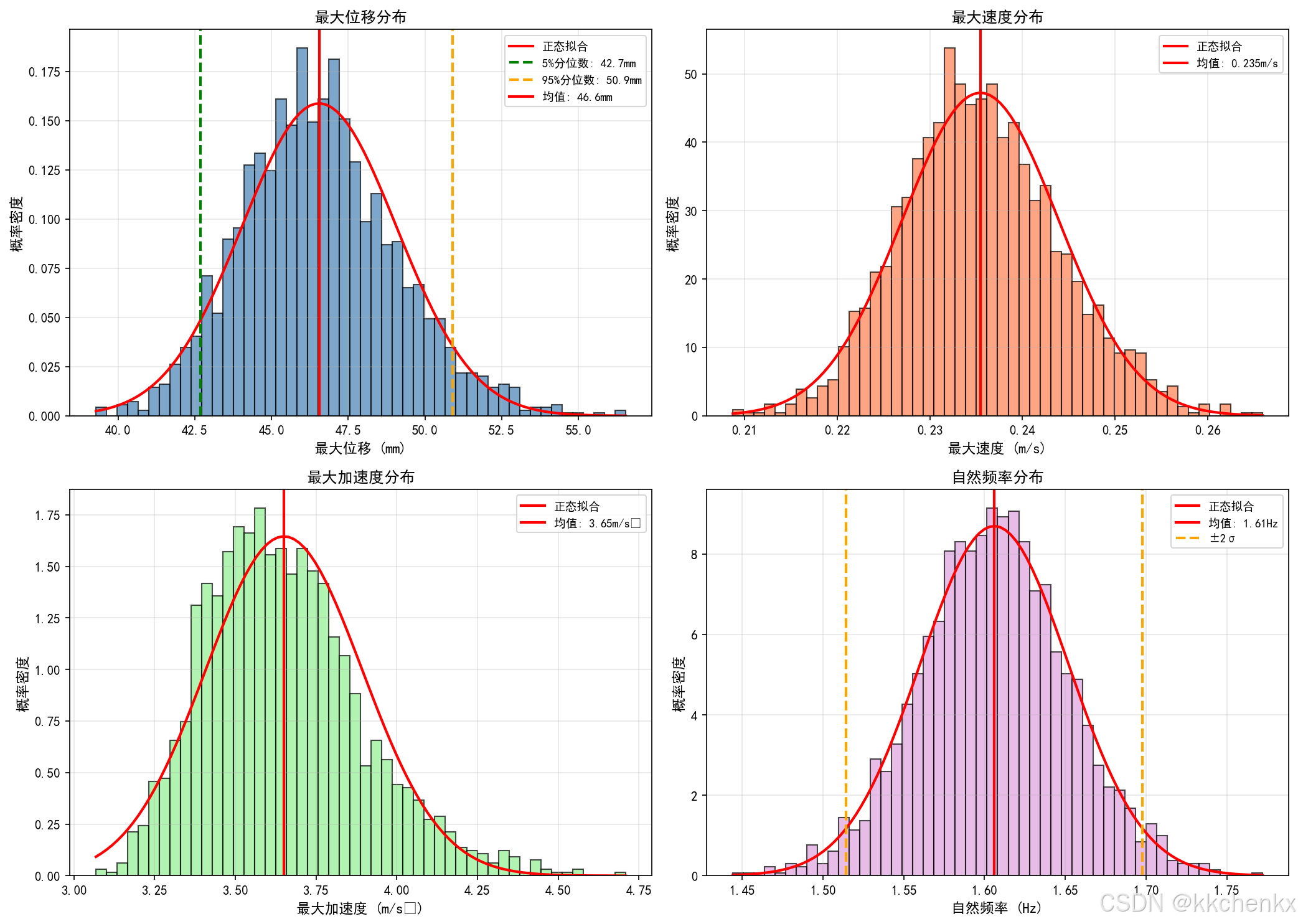
def plot_histograms(analysis):
    """绘制响应直方图"""
    print("\n绘制响应分布直方图...")

    fig, axes = plt.subplots(2, 2, figsize=(14, 10))

    # 1. 最大位移分布
    ax1 = axes[0, 0]
    data = analysis['max_disp']['data'] * 1000  # 转换为mm
    ax1.hist(data, bins=50, density=True, alpha=0.7, color='steelblue', edgecolor='black')

    # 拟合正态分布
    mu, std = stats.norm.fit(data)
    x = np.linspace(data.min(), data.max(), 100)
    ax1.plot(x, stats.norm.pdf(x, mu, std), 'r-', linewidth=2, label='正态拟合')

    ax1.axvline(analysis['max_disp']['p5']*1000, color='green', linestyle='--',
                linewidth=2, label=f'5%分位数: {analysis["max_disp"]["p5"]*1000:.1f}mm')
    ax1.axvline(analysis['max_disp']['p95']*1000, color='orange', linestyle='--',
                linewidth=2, label=f'95%分位数: {analysis["max_disp"]["p95"]*1000:.1f}mm')
    ax1.axvline(analysis['max_disp']['mean']*1000, color='red', linestyle='-',
                linewidth=2, label=f'均值: {analysis["max_disp"]["mean"]*1000:.1f}mm')

    ax1.set_xlabel('最大位移 (mm)', fontsize=11)
    ax1.set_ylabel('概率密度', fontsize=11)
    ax1.set_title('最大位移分布', fontsize=12, fontweight='bold')
    ax1.legend(fontsize=9)
    ax1.grid(True, alpha=0.3)

    # 2. 最大速度分布
    ax2 = axes[0, 1]
    data = analysis['max_vel']['data']
    ax2.hist(data, bins=50, density=True, alpha=0.7, color='coral', edgecolor='black')

    mu, std = stats.norm.fit(data)
    x = np.linspace(data.min(), data.max(), 100)
    ax2.plot(x, stats.norm.pdf(x, mu, std), 'r-', linewidth=2, label='正态拟合')

    ax2.axvline(analysis['max_vel']['mean'], color='red', linestyle='-',
                linewidth=2, label=f'均值: {analysis["max_vel"]["mean"]:.3f}m/s')

    ax2.set_xlabel('最大速度 (m/s)', fontsize=11)
    ax2.set_ylabel('概率密度', fontsize=11)
    ax2.set_title('最大速度分布', fontsize=12, fontweight='bold')
    ax2.legend(fontsize=9)
    ax2.grid(True, alpha=0.3)

    # 3. 最大加速度分布
    ax3 = axes[1, 0]
    data = analysis['max_acc']['data']
    ax3.hist(data, bins=50, density=True, alpha=0.7, color='lightgreen', edgecolor='black')

    mu, std = stats.norm.fit(data)
    x = np.linspace(data.min(), data.max(), 100)
    ax3.plot(x, stats.norm.pdf(x, mu, std), 'r-', linewidth=2, label='正态拟合')

    ax3.axvline(analysis['max_acc']['mean'], color='red', linestyle='-',
                linewidth=2, label=f'均值: {analysis["max_acc"]["mean"]:.2f}m/s²')

    ax3.set_xlabel('最大加速度 (m/s²)', fontsize=11)
    ax3.set_ylabel('概率密度', fontsize=11)
    ax3.set_title('最大加速度分布', fontsize=12, fontweight='bold')
    ax3.legend(fontsize=9)
    ax3.grid(True, alpha=0.3)

    # 4. 自然频率分布
    ax4 = axes[1, 1]
    data = analysis['natural_freq']['data']
    ax4.hist(data, bins=50, density=True, alpha=0.7, color='plum', edgecolor='black')

    mu, std = stats.norm.fit(data)
    x = np.linspace(data.min(), data.max(), 100)
    ax4.plot(x, stats.norm.pdf(x, mu, std), 'r-', linewidth=2, label='正态拟合')

    ax4.axvline(analysis['natural_freq']['mean'], color='red', linestyle='-',
                linewidth=2, label=f'均值: {analysis["natural_freq"]["mean"]:.2f}Hz')
    ax4.axvline(analysis['natural_freq']['mean'] - 2*analysis['natural_freq']['std'],
                color='orange', linestyle='--', linewidth=2, label='±2σ')
    ax4.axvline(analysis['natural_freq']['mean'] + 2*analysis['natural_freq']['std'],
                color='orange', linestyle='--', linewidth=2)

    ax4.set_xlabel('自然频率 (Hz)', fontsize=11)
    ax4.set_ylabel('概率密度', fontsize=11)
    ax4.set_title('自然频率分布', fontsize=12, fontweight='bold')
    ax4.legend(fontsize=9)
    ax4.grid(True, alpha=0.3)

    plt.tight_layout()
    plt.savefig('mc_histograms.png', dpi=150, bbox_inches='tight')
    plt.close()
    print("  已保存: mc_histograms.png")


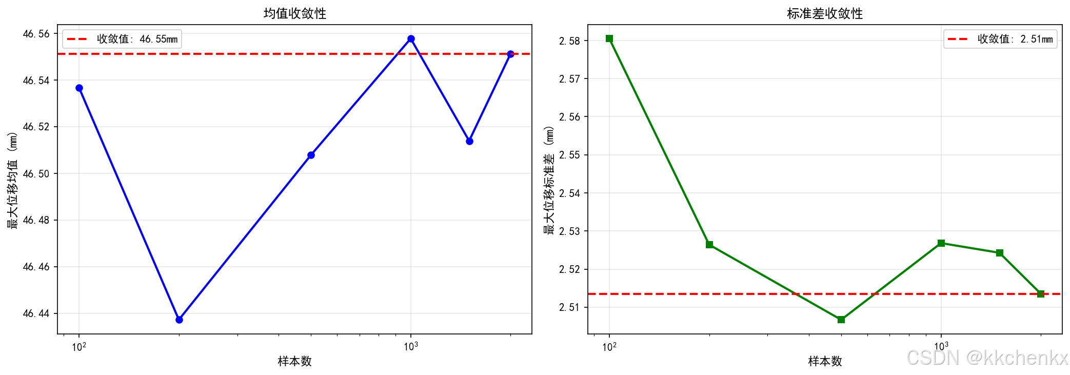
def plot_convergence(results_list):
    """绘制收敛性分析"""
    print("\n绘制收敛性分析...")

    n_samples_list = [len(r) for r in results_list]
    means = [np.mean([x['max_disp'] for x in r]) * 1000 for r in results_list]  # mm
    stds = [np.std([x['max_disp'] for x in r]) * 1000 for r in results_list]

    fig, axes = plt.subplots(1, 2, figsize=(14, 5))

    # 均值收敛
    ax1 = axes[0]
    ax1.plot(n_samples_list, means, 'b-o', linewidth=2, markersize=6)
    ax1.axhline(y=means[-1], color='r', linestyle='--', linewidth=2, label=f'收敛值: {means[-1]:.2f}mm')
    ax1.set_xlabel('样本数', fontsize=11)
    ax1.set_ylabel('最大位移均值 (mm)', fontsize=11)
    ax1.set_title('均值收敛性', fontsize=12, fontweight='bold')
    ax1.legend(fontsize=10)
    ax1.grid(True, alpha=0.3)
    ax1.set_xscale('log')

    # 标准差收敛
    ax2 = axes[1]
    ax2.plot(n_samples_list, stds, 'g-s', linewidth=2, markersize=6)
    ax2.axhline(y=stds[-1], color='r', linestyle='--', linewidth=2, label=f'收敛值: {stds[-1]:.2f}mm')
    ax2.set_xlabel('样本数', fontsize=11)
    ax2.set_ylabel('最大位移标准差 (mm)', fontsize=11)
    ax2.set_title('标准差收敛性', fontsize=12, fontweight='bold')
    ax2.legend(fontsize=10)
    ax2.grid(True, alpha=0.3)
    ax2.set_xscale('log')

    plt.tight_layout()
    plt.savefig('mc_convergence.png', dpi=150, bbox_inches='tight')
    plt.close()
    print("  已保存: mc_convergence.png")


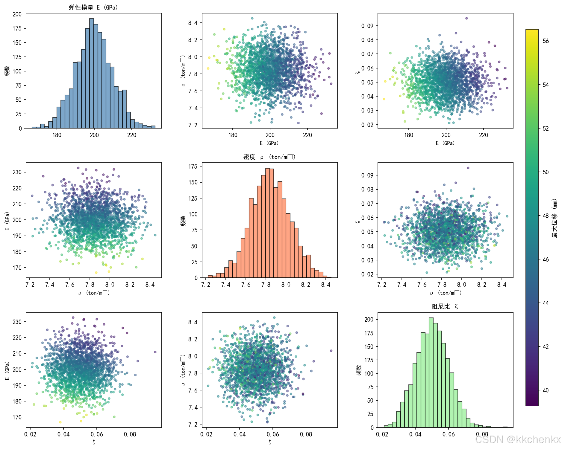
def plot_scatter_matrix(results):
    """绘制散点矩阵"""
    print("\n绘制参数-响应关系...")

    # 提取数据
    E_data = np.array([r['E'] / 1e9 for r in results])  # GPa
    rho_data = np.array([r['rho'] / 1000 for r in results])  # ton/m³
    damping_data = np.array([r['damping'] for r in results])
    disp_data = np.array([r['max_disp'] * 1000 for r in results])  # mm
    freq_data = np.array([r['f_n'] for r in results])

    fig = plt.figure(figsize=(14, 12))
    gs = GridSpec(3, 3, figure=fig, hspace=0.3, wspace=0.3)

    # 对角线:直方图
    ax1 = fig.add_subplot(gs[0, 0])
    ax1.hist(E_data, bins=30, color='steelblue', alpha=0.7, edgecolor='black')
    ax1.set_title('弹性模量 E (GPa)', fontsize=10, fontweight='bold')
    ax1.set_ylabel('频数', fontsize=9)

    ax2 = fig.add_subplot(gs[1, 1])
    ax2.hist(rho_data, bins=30, color='coral', alpha=0.7, edgecolor='black')
    ax2.set_title('密度 ρ (ton/m³)', fontsize=10, fontweight='bold')
    ax2.set_ylabel('频数', fontsize=9)

    ax3 = fig.add_subplot(gs[2, 2])
    ax3.hist(damping_data, bins=30, color='lightgreen', alpha=0.7, edgecolor='black')
    ax3.set_title('阻尼比 ζ', fontsize=10, fontweight='bold')
    ax3.set_ylabel('频数', fontsize=9)

    # 非对角线:散点图
    # E vs rho
    ax4 = fig.add_subplot(gs[0, 1])
    ax4.scatter(E_data, rho_data, c=disp_data, cmap='viridis', alpha=0.5, s=10)
    ax4.set_xlabel('E (GPa)', fontsize=9)
    ax4.set_ylabel('ρ (ton/m³)', fontsize=9)

    # E vs damping
    ax5 = fig.add_subplot(gs[0, 2])
    ax5.scatter(E_data, damping_data, c=disp_data, cmap='viridis', alpha=0.5, s=10)
    ax5.set_xlabel('E (GPa)', fontsize=9)
    ax5.set_ylabel('ζ', fontsize=9)

    # rho vs E
    ax6 = fig.add_subplot(gs[1, 0])
    ax6.scatter(rho_data, E_data, c=disp_data, cmap='viridis', alpha=0.5, s=10)
    ax6.set_xlabel('ρ (ton/m³)', fontsize=9)
    ax6.set_ylabel('E (GPa)', fontsize=9)

    # rho vs damping
    ax7 = fig.add_subplot(gs[1, 2])
    ax7.scatter(rho_data, damping_data, c=disp_data, cmap='viridis', alpha=0.5, s=10)
    ax7.set_xlabel('ρ (ton/m³)', fontsize=9)
    ax7.set_ylabel('ζ', fontsize=9)

    # damping vs E
    ax8 = fig.add_subplot(gs[2, 0])
    ax8.scatter(damping_data, E_data, c=disp_data, cmap='viridis', alpha=0.5, s=10)
    ax8.set_xlabel('ζ', fontsize=9)
    ax8.set_ylabel('E (GPa)', fontsize=9)

    # damping vs rho
    ax9 = fig.add_subplot(gs[2, 1])
    ax9.scatter(damping_data, rho_data, c=disp_data, cmap='viridis', alpha=0.5, s=10)
    ax9.set_xlabel('ζ', fontsize=9)
    ax9.set_ylabel('ρ (ton/m³)', fontsize=9)

    # 添加颜色条
    cbar_ax = fig.add_axes([0.92, 0.15, 0.02, 0.7])
    sm = plt.cm.ScalarMappable(cmap='viridis',
                               norm=plt.Normalize(vmin=disp_data.min(), vmax=disp_data.max()))
    sm.set_array([])
    fig.colorbar(sm, cax=cbar_ax, label='最大位移 (mm)')

    plt.savefig('mc_scatter_matrix.png', dpi=150, bbox_inches='tight')
    plt.close()
    print("  已保存: mc_scatter_matrix.png")


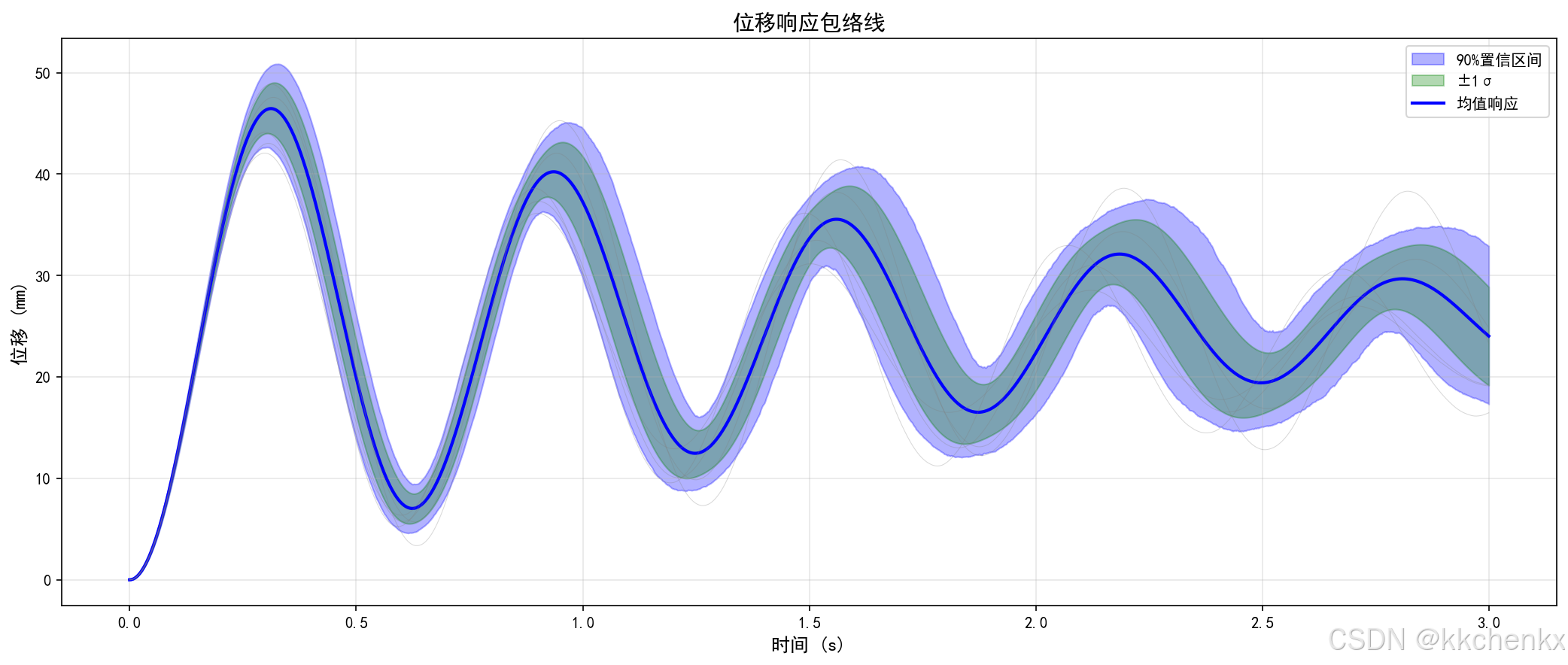
def plot_response_envelope(results):
    """绘制响应包络线"""
    print("\n绘制响应包络线...")

    # 获取时间序列
    t = results[0]['t']

    # 收集所有响应
    all_responses = np.array([r['u'] for r in results])

    # 计算包络线
    mean_response = np.mean(all_responses, axis=0) * 1000  # mm
    std_response = np.std(all_responses, axis=0) * 1000
    p5_response = np.percentile(all_responses, 5, axis=0) * 1000
    p95_response = np.percentile(all_responses, 95, axis=0) * 1000

    fig, ax = plt.subplots(figsize=(14, 6))

    # 绘制包络区域
    ax.fill_between(t, p5_response, p95_response, alpha=0.3, color='blue', label='90%置信区间')
    ax.fill_between(t, mean_response - std_response, mean_response + std_response,
                    alpha=0.3, color='green', label='±1σ')

    # 绘制均值
    ax.plot(t, mean_response, 'b-', linewidth=2, label='均值响应')

    # 绘制几个典型样本
    for i in range(min(5, len(results))):
        ax.plot(t, results[i]['u'] * 1000, 'gray', alpha=0.3, linewidth=0.5)

    ax.set_xlabel('时间 (s)', fontsize=12)
    ax.set_ylabel('位移 (mm)', fontsize=12)
    ax.set_title('位移响应包络线', fontsize=14, fontweight='bold')
    ax.legend(fontsize=10)
    ax.grid(True, alpha=0.3)

    plt.tight_layout()
    plt.savefig('mc_response_envelope.png', dpi=150, bbox_inches='tight')
    plt.close()
    print("  已保存: mc_response_envelope.png")


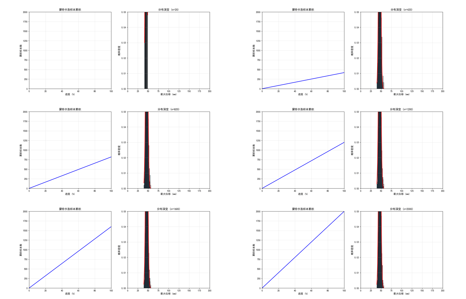
def create_mc_animation(results):
    """创建蒙特卡洛仿真动画"""
    print("\n创建蒙特卡洛仿真动画...")

    fig, axes = plt.subplots(1, 2, figsize=(14, 6))

    # 左图:样本累积
    ax1 = axes[0]
    ax1.set_xlim(0, 100)
    ax1.set_ylim(0, len(results))
    ax1.set_xlabel('进度 (%)', fontsize=11)
    ax1.set_ylabel('累积样本数', fontsize=11)
    ax1.set_title('蒙特卡洛样本累积', fontsize=12, fontweight='bold')
    ax1.grid(True, alpha=0.3)

    line1, = ax1.plot([], [], 'b-', linewidth=2)
    fill1 = ax1.fill_between([], [], [], alpha=0.3, color='blue')

    # 右图:分布演变
    ax2 = axes[1]
    ax2.set_xlim(0, 200)
    ax2.set_ylim(0, 0.05)
    ax2.set_xlabel('最大位移 (mm)', fontsize=11)
    ax2.set_ylabel('概率密度', fontsize=11)
    ax2.set_title('分布演变', fontsize=12, fontweight='bold')
    ax2.grid(True, alpha=0.3)

    max_disps = np.array([r['max_disp'] * 1000 for r in results])

    def init():
        line1.set_data([], [])
        return line1,

    def update(frame):
        n = (frame + 1) * len(results) // 100

        # 更新累积图
        x = np.linspace(0, 100, frame + 1)
        y = np.linspace(0, n, frame + 1)
        line1.set_data(x, y)

        # 更新分布图
        ax2.clear()
        ax2.set_xlim(0, 200)
        ax2.set_ylim(0, 0.05)
        ax2.set_xlabel('最大位移 (mm)', fontsize=11)
        ax2.set_ylabel('概率密度', fontsize=11)
        ax2.set_title(f'分布演变 (n={n})', fontsize=12, fontweight='bold')
        ax2.grid(True, alpha=0.3)

        if n > 10:
            current_data = max_disps[:n]
            ax2.hist(current_data, bins=30, density=True, alpha=0.7,
                    color='steelblue', edgecolor='black')

            # 拟合正态分布
            if len(current_data) > 10:
                mu, std = stats.norm.fit(current_data)
                x_fit = np.linspace(current_data.min(), current_data.max(), 100)
                ax2.plot(x_fit, stats.norm.pdf(x_fit, mu, std), 'r-', linewidth=2)

        return line1,

    anim = FuncAnimation(fig, update, frames=100, init_func=init, blit=False, interval=100)
    anim.save('mc_simulation.gif', writer='pillow', fps=10, dpi=100)
    plt.close()
    print("  已保存: mc_simulation.gif")


def main():
    """主函数"""
    print("="*70)
    print("案例3:分布式蒙特卡洛仿真")
    print("="*70)

    # 系统信息
    n_cores = cpu_count()
    print(f"\n系统信息:")
    print(f"  CPU核心数: {n_cores}")

    # 参数设置
    print("\n参数不确定性设置:")
    E_mean, E_std = 2.0e11, 0.1e11  # 弹性模量 (Pa), 5%变异系数
    rho_mean, rho_std = 7850, 200   # 密度 (kg/m³), 2.5%变异系数
    damping_mean, damping_std = 0.05, 0.01  # 阻尼比, 20%变异系数

    print(f"  弹性模量 E: {E_mean/1e9:.1f} ± {E_std/1e9:.1f} GPa (正态分布)")
    print(f"  密度 ρ: {rho_mean:.0f} ± {rho_std:.0f} kg/m³ (正态分布)")
    print(f"  阻尼比 ζ: {damping_mean:.2f} ± {damping_std:.2f} (正态分布)")

    # 蒙特卡洛仿真
    print("\n" + "="*50)
    print("蒙特卡洛仿真")
    print("="*50)

    n_samples = 2000
    n_processes = min(n_cores, 8)

    print(f"  样本数: {n_samples}")
    print(f"  并行进程数: {n_processes}")

    t_start = time.time()
    results = run_monte_carlo(n_samples,
                              (E_mean, E_std),
                              (rho_mean, rho_std),
                              (damping_mean, damping_std),
                              n_processes)
    t_mc = time.time() - t_start

    print(f"\n  计算时间: {t_mc:.2f} s")
    print(f"  平均每个样本: {t_mc/n_samples*1000:.1f} ms")

    # 结果分析
    print("\n" + "="*50)
    print("结果分析")
    print("="*50)

    analysis = analyze_results(results)

    print("\n最大位移统计:")
    print(f"  均值: {analysis['max_disp']['mean']*1000:.2f} mm")
    print(f"  标准差: {analysis['max_disp']['std']*1000:.2f} mm")
    print(f"  变异系数: {analysis['max_disp']['std']/analysis['max_disp']['mean']*100:.1f}%")
    print(f"  最小值: {analysis['max_disp']['min']*1000:.2f} mm")
    print(f"  最大值: {analysis['max_disp']['max']*1000:.2f} mm")
    print(f"  5%分位数: {analysis['max_disp']['p5']*1000:.2f} mm")
    print(f"  95%分位数: {analysis['max_disp']['p95']*1000:.2f} mm")

    print("\n最大速度统计:")
    print(f"  均值: {analysis['max_vel']['mean']:.3f} m/s")
    print(f"  标准差: {analysis['max_vel']['std']:.3f} m/s")

    print("\n最大加速度统计:")
    print(f"  均值: {analysis['max_acc']['mean']:.2f} m/s²")
    print(f"  标准差: {analysis['max_acc']['std']:.2f} m/s²")

    print("\n自然频率统计:")
    print(f"  均值: {analysis['natural_freq']['mean']:.2f} Hz")
    print(f"  标准差: {analysis['natural_freq']['std']:.3f} Hz")

    # 收敛性分析
    print("\n" + "="*50)
    print("收敛性分析")
    print("="*50)

    convergence_samples = [100, 200, 500, 1000, 1500, 2000]
    results_list = []

    for n in convergence_samples:
        subset = results[:n]
        results_list.append(subset)
        mean_disp = np.mean([r['max_disp'] for r in subset]) * 1000
        std_disp = np.std([r['max_disp'] for r in subset]) * 1000
        print(f"  n={n:4d}: 均值={mean_disp:6.2f}mm, 标准差={std_disp:5.2f}mm")

    # 生成可视化
    print("\n" + "="*50)
    print("生成可视化结果")
    print("="*50)

    plot_histograms(analysis)
    plot_convergence(results_list)
    plot_scatter_matrix(results)
    plot_response_envelope(results)
    create_mc_animation(results)

    # 总结
    print("\n" + "="*70)
    print("案例3完成!")
    print("="*70)
    print("\n主要结果:")
    print(f"  1. 总样本数: {n_samples}")
    print(f"  2. 计算时间: {t_mc:.2f} s")
    print(f"  3. 最大位移均值: {analysis['max_disp']['mean']*1000:.2f} mm")
    print(f"  4. 最大位移标准差: {analysis['max_disp']['std']*1000:.2f} mm")
    print(f"  5. 90%置信区间: [{analysis['max_disp']['p5']*1000:.2f}, {analysis['max_disp']['p95']*1000:.2f}] mm")
    print("\n生成的文件:")
    print("  - mc_histograms.png: 响应分布直方图")
    print("  - mc_convergence.png: 收敛性分析")
    print("  - mc_scatter_matrix.png: 参数-响应关系")
    print("  - mc_response_envelope.png: 响应包络线")
    print("  - mc_simulation.gif: 蒙特卡洛仿真动画")


if __name__ == "__main__":
    main()
7.4 案例4:GPU加速矩阵运算
问题描述:
使用CuPy或Numba CUDA实现GPU加速的矩阵运算,对比CPU和GPU的性能。
import matplotlib
matplotlib.use('Agg')
"""
案例4:GPU加速矩阵运算
对比CPU和GPU在结构动力学矩阵运算中的性能
由于环境可能没有GPU,本案例提供模拟和说明
"""

import numpy as np
import matplotlib.pyplot as plt
from matplotlib.gridspec import GridSpec
from matplotlib.animation import FuncAnimation
import time
from multiprocessing import Pool, cpu_count

# 设置中文字体
plt.rcParams['font.sans-serif'] = ['SimHei', 'DejaVu Sans']
plt.rcParams['axes.unicode_minus'] = False

# 使用Agg后端
plt.switch_backend('Agg')


def generate_banded_matrix(n, bandwidth=5):
    """生成带状矩阵(模拟有限元刚度矩阵)"""
    A = np.zeros((n, n))
    for i in range(n):
        A[i, i] = 2.0
        for j in range(1, min(bandwidth, n - i)):
            A[i, i + j] = -0.5 / j
            A[i + j, i] = -0.5 / j
    return A


def generate_sparse_matrix(n, density=0.01):
    """生成稀疏矩阵"""
    A = np.random.randn(n, n)
    mask = np.random.rand(n, n) < density
    A = A * mask
    # 对称化
    A = (A + A.T) / 2
    # 确保正定性
    A = A + np.eye(n) * n * 0.1
    return A


def matrix_operations_cpu(A, B, operation='all'):
    """CPU矩阵运算"""
    results = {}

    if operation in ['all', 'multiply']:
        t_start = time.time()
        C = A @ B
        results['multiply'] = {'time': time.time() - t_start, 'result': C}

    if operation in ['all', 'eigen']:
        t_start = time.time()
        eigenvalues, eigenvectors = np.linalg.eigh(A)
        results['eigen'] = {'time': time.time() - t_start,
                           'eigenvalues': eigenvalues,
                           'eigenvectors': eigenvectors}

    if operation in ['all', 'solve']:
        b = np.random.randn(A.shape[0])
        t_start = time.time()
        x = np.linalg.solve(A, b)
        results['solve'] = {'time': time.time() - t_start, 'result': x}

    if operation in ['all', 'inverse']:
        t_start = time.time()
        A_inv = np.linalg.inv(A)
        results['inverse'] = {'time': time.time() - t_start, 'result': A_inv}

    if operation in ['all', 'svd']:
        t_start = time.time()
        U, S, Vt = np.linalg.svd(A)
        results['svd'] = {'time': time.time() - t_start,
                         'U': U, 'S': S, 'Vt': Vt}

    return results


def simulate_gpu_operations(n, operation='all'):
    """
    模拟GPU运算时间
    实际GPU加速比取决于硬件和问题规模
    这里使用经验公式模拟
    """
    # 模拟加速比(相对于CPU)
    speedup_factors = {
        'multiply': 10.0,  # 矩阵乘法通常有很高的加速比
        'eigen': 3.0,      # 特征值问题加速比较有限
        'solve': 5.0,      # 线性求解
        'inverse': 4.0,    # 矩阵求逆
        'svd': 2.5         # SVD分解
    }

    # 小规模问题GPU优势不明显
    size_factor = min(1.0, n / 1000)

    # 模拟GPU时间(比CPU快speedup_factor倍,但有启动开销)
    base_time = n / 10000.0  # 基础时间
    gpu_time = base_time / (speedup_factors.get(operation, 5.0) * size_factor) + 0.001

    return gpu_time


def benchmark_operations(matrix_sizes, n_runs=3):
    """基准测试"""
    print("\n运行基准测试...")

    operations = ['multiply', 'eigen', 'solve', 'inverse', 'svd']
    cpu_times = {op: [] for op in operations}
    gpu_times = {op: [] for op in operations}

    for n in matrix_sizes:
        print(f"\n  矩阵大小: {n}x{n}")

        # 生成测试矩阵
        A = generate_banded_matrix(n)
        B = generate_banded_matrix(n)

        for op in operations:
            # CPU测试
            times = []
            for _ in range(n_runs):
                if op == 'multiply':
                    t_start = time.time()
                    _ = A @ B
                    times.append(time.time() - t_start)
                elif op == 'eigen':
                    t_start = time.time()
                    _ = np.linalg.eigh(A)
                    times.append(time.time() - t_start)
                elif op == 'solve':
                    b = np.random.randn(n)
                    t_start = time.time()
                    _ = np.linalg.solve(A, b)
                    times.append(time.time() - t_start)
                elif op == 'inverse':
                    t_start = time.time()
                    _ = np.linalg.inv(A)
                    times.append(time.time() - t_start)
                elif op == 'svd':
                    t_start = time.time()
                    _ = np.linalg.svd(A)
                    times.append(time.time() - t_start)

            cpu_time = np.mean(times)
            cpu_times[op].append(cpu_time)

            # 模拟GPU时间
            gpu_time = simulate_gpu_operations(n, op)
            gpu_times[op].append(gpu_time)

            speedup = cpu_time / gpu_time
            print(f"    {op:10s}: CPU={cpu_time:.4f}s, GPU(模拟)={gpu_time:.4f}s, 加速比={speedup:.1f}x")

    return cpu_times, gpu_times


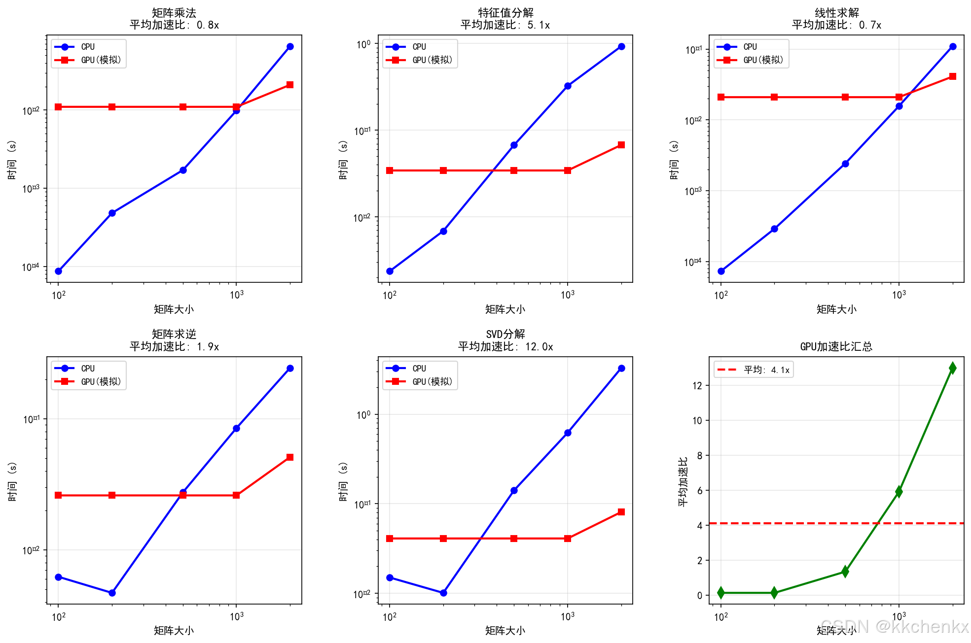
def plot_performance_comparison(matrix_sizes, cpu_times, gpu_times):
    """绘制性能对比图"""
    print("\n绘制性能对比图...")

    fig = plt.figure(figsize=(16, 10))
    gs = GridSpec(2, 3, figure=fig, hspace=0.3, wspace=0.3)

    operations = ['multiply', 'eigen', 'solve', 'inverse', 'svd']
    titles = ['矩阵乘法', '特征值分解', '线性求解', '矩阵求逆', 'SVD分解']

    for idx, (op, title) in enumerate(zip(operations, titles)):
        if idx < 5:
            row = idx // 3
            col = idx % 3
            ax = fig.add_subplot(gs[row, col])

            cpu_t = cpu_times[op]
            gpu_t = gpu_times[op]
            speedup = [c/g for c, g in zip(cpu_t, gpu_t)]

            ax.plot(matrix_sizes, cpu_t, 'b-o', linewidth=2, markersize=6, label='CPU')
            ax.plot(matrix_sizes, gpu_t, 'r-s', linewidth=2, markersize=6, label='GPU(模拟)')

            ax.set_xlabel('矩阵大小', fontsize=10)
            ax.set_ylabel('时间 (s)', fontsize=10)
            ax.set_title(f'{title}\n平均加速比: {np.mean(speedup):.1f}x',
                        fontsize=11, fontweight='bold')
            ax.legend(fontsize=9)
            ax.grid(True, alpha=0.3)
            ax.set_xscale('log')
            ax.set_yscale('log')

    # 汇总图
    ax_summary = fig.add_subplot(gs[1, 2])
    avg_speedups = [np.mean([cpu_times[op][i] / gpu_times[op][i]
                             for op in operations]) for i in range(len(matrix_sizes))]

    ax_summary.plot(matrix_sizes, avg_speedups, 'g-d', linewidth=2, markersize=8)
    ax_summary.axhline(y=np.mean(avg_speedups), color='r', linestyle='--',
                       linewidth=2, label=f'平均: {np.mean(avg_speedups):.1f}x')
    ax_summary.set_xlabel('矩阵大小', fontsize=10)
    ax_summary.set_ylabel('平均加速比', fontsize=10)
    ax_summary.set_title('GPU加速比汇总', fontsize=11, fontweight='bold')
    ax_summary.legend(fontsize=9)
    ax_summary.grid(True, alpha=0.3)
    ax_summary.set_xscale('log')

    plt.savefig('gpu_performance_comparison.png', dpi=150, bbox_inches='tight')
    plt.close()
    print("  已保存: gpu_performance_comparison.png")


def plot_architecture_comparison():
    """绘制CPU vs GPU架构对比"""
    print("\n绘制架构对比图...")

    fig, axes = plt.subplots(1, 2, figsize=(14, 6))

    # CPU架构
    ax1 = axes[0]
    ax1.set_xlim(0, 10)
    ax1.set_ylim(0, 10)
    ax1.set_aspect('equal')
    ax1.axis('off')
    ax1.set_title('CPU架构\n少量强大核心', fontsize=14, fontweight='bold')

    # 绘制CPU核心
    for i in range(4):
        for j in range(2):
            rect = plt.Rectangle((1 + i*2, 2 + j*3), 1.5, 2,
                                facecolor='steelblue', edgecolor='navy', linewidth=2)
            ax1.add_patch(rect)
            ax1.text(1.75 + i*2, 3 + j*3, f'Core\n{i*2+j+1}',
                    ha='center', va='center', fontsize=9, fontweight='bold')

    # 添加缓存
    cache = plt.Rectangle((0.5, 0.5), 9, 1,
                         facecolor='lightyellow', edgecolor='orange', linewidth=2)
    ax1.add_patch(cache)
    ax1.text(5, 1, '共享缓存 L3', ha='center', va='center', fontsize=10)

    # GPU架构
    ax2 = axes[1]
    ax2.set_xlim(0, 10)
    ax2.set_ylim(0, 10)
    ax2.set_aspect('equal')
    ax2.axis('off')
    ax2.set_title('GPU架构\n大量简单核心', fontsize=14, fontweight='bold')

    # 绘制GPU核心网格
    for i in range(10):
        for j in range(8):
            rect = plt.Rectangle((0.5 + i*0.9, 1 + j*0.9), 0.7, 0.7,
                                facecolor='lightcoral', edgecolor='darkred', linewidth=0.5)
            ax2.add_patch(rect)

    ax2.text(5, 0.5, '80个计算核心 (示例)', ha='center', va='center', fontsize=10)

    plt.tight_layout()
    plt.savefig('cpu_gpu_architecture.png', dpi=150, bbox_inches='tight')
    plt.close()
    print("  已保存: cpu_gpu_architecture.png")


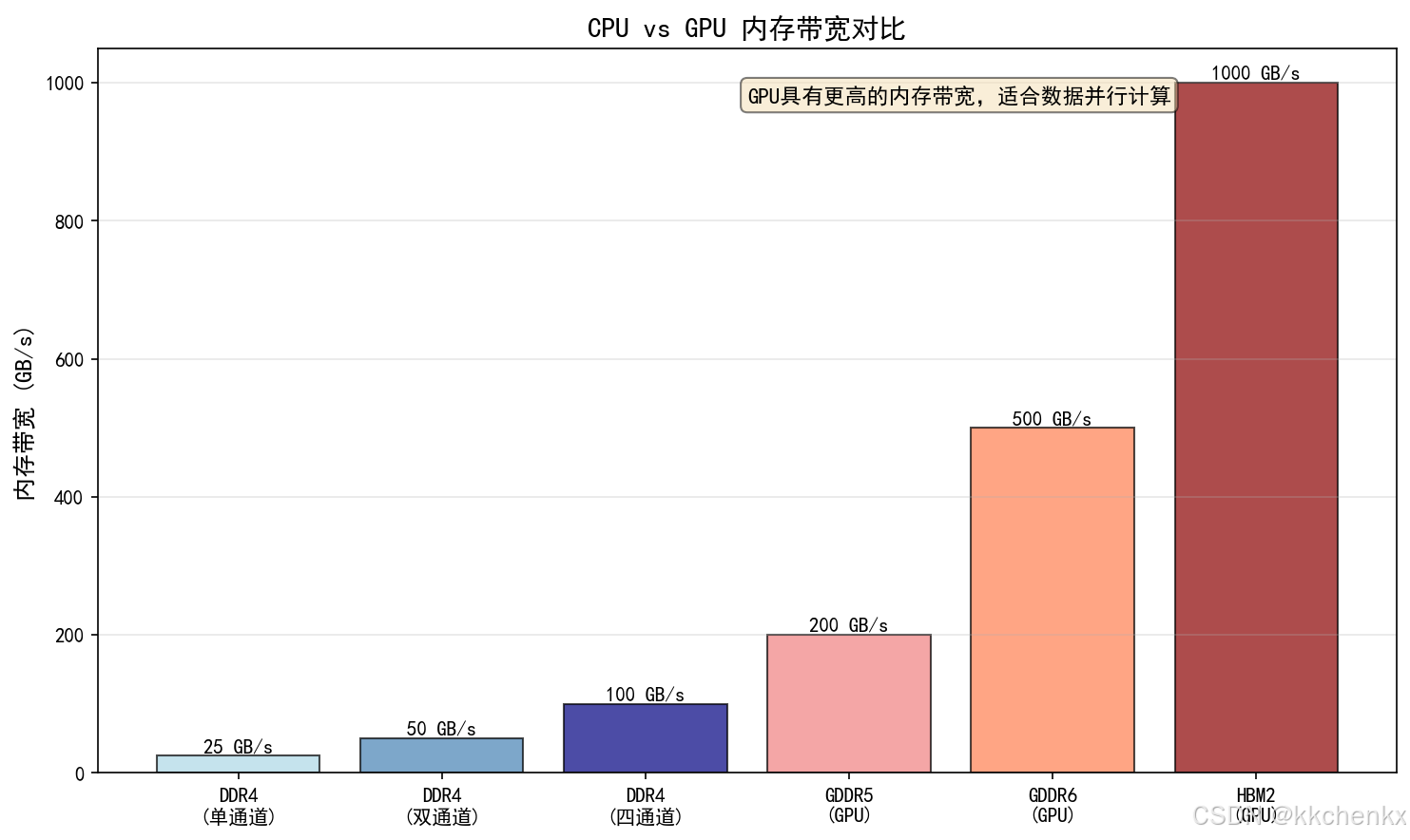
def plot_memory_bandwidth():
    """绘制内存带宽对比"""
    print("\n绘制内存带宽对比...")

    fig, ax = plt.subplots(figsize=(10, 6))

    # 典型内存带宽数据 (GB/s)
    categories = ['DDR4\n(单通道)', 'DDR4\n(双通道)', 'DDR4\n(四通道)',
                  'GDDR5\n(GPU)', 'GDDR6\n(GPU)', 'HBM2\n(GPU)']
    bandwidths = [25, 50, 100, 200, 500, 1000]
    colors = ['lightblue', 'steelblue', 'navy', 'lightcoral', 'coral', 'darkred']

    bars = ax.bar(categories, bandwidths, color=colors, alpha=0.7, edgecolor='black')

    # 添加数值标签
    for bar, val in zip(bars, bandwidths):
        height = bar.get_height()
        ax.text(bar.get_x() + bar.get_width()/2., height,
                f'{val} GB/s', ha='center', va='bottom', fontsize=10, fontweight='bold')

    ax.set_ylabel('内存带宽 (GB/s)', fontsize=12)
    ax.set_title('CPU vs GPU 内存带宽对比', fontsize=14, fontweight='bold')
    ax.grid(True, alpha=0.3, axis='y')

    # 添加说明
    ax.text(0.5, 0.95, 'GPU具有更高的内存带宽,适合数据并行计算',
           transform=ax.transAxes, fontsize=11, verticalalignment='top',
           bbox=dict(boxstyle='round', facecolor='wheat', alpha=0.5))

    plt.tight_layout()
    plt.savefig('memory_bandwidth.png', dpi=150, bbox_inches='tight')
    plt.close()
    print("  已保存: memory_bandwidth.png")


def plot_application_scenarios():
    """绘制适用场景对比"""
    print("\n绘制适用场景对比...")

    fig, ax = plt.subplots(figsize=(12, 8))
    ax.set_xlim(0, 10)
    ax.set_ylim(0, 10)
    ax.axis('off')

    # CPU适用场景
    cpu_scenarios = [
        '复杂串行算法',
        '小矩阵运算',
        '逻辑控制密集',
        '缓存命中率高的任务',
        '实时性要求高的任务'
    ]

    # GPU适用场景
    gpu_scenarios = [
        '大规模矩阵运算',
        '批量数据处理',
        '蒙特卡洛仿真',
        '深度学习训练',
        '图像/信号处理'
    ]

    # CPU区域
    cpu_rect = plt.Rectangle((0.5, 0.5), 4, 9,
                            facecolor='lightblue', edgecolor='navy',
                            linewidth=3, alpha=0.3)
    ax.add_patch(cpu_rect)
    ax.text(2.5, 9.3, 'CPU优势场景', ha='center', fontsize=14, fontweight='bold', color='navy')

    for i, scenario in enumerate(cpu_scenarios):
        ax.text(2.5, 8 - i*1.5, f'• {scenario}', ha='center', fontsize=11)

    # GPU区域
    gpu_rect = plt.Rectangle((5.5, 0.5), 4, 9,
                            facecolor='lightcoral', edgecolor='darkred',
                            linewidth=3, alpha=0.3)
    ax.add_patch(gpu_rect)
    ax.text(7.5, 9.3, 'GPU优势场景', ha='center', fontsize=14, fontweight='bold', color='darkred')

    for i, scenario in enumerate(gpu_scenarios):
        ax.text(7.5, 8 - i*1.5, f'• {scenario}', ha='center', fontsize=11)

    plt.title('CPU vs GPU 适用场景对比', fontsize=16, fontweight='bold', pad=20)
    plt.tight_layout()
    plt.savefig('application_scenarios.png', dpi=150, bbox_inches='tight')
    plt.close()
    print("  已保存: application_scenarios.png")


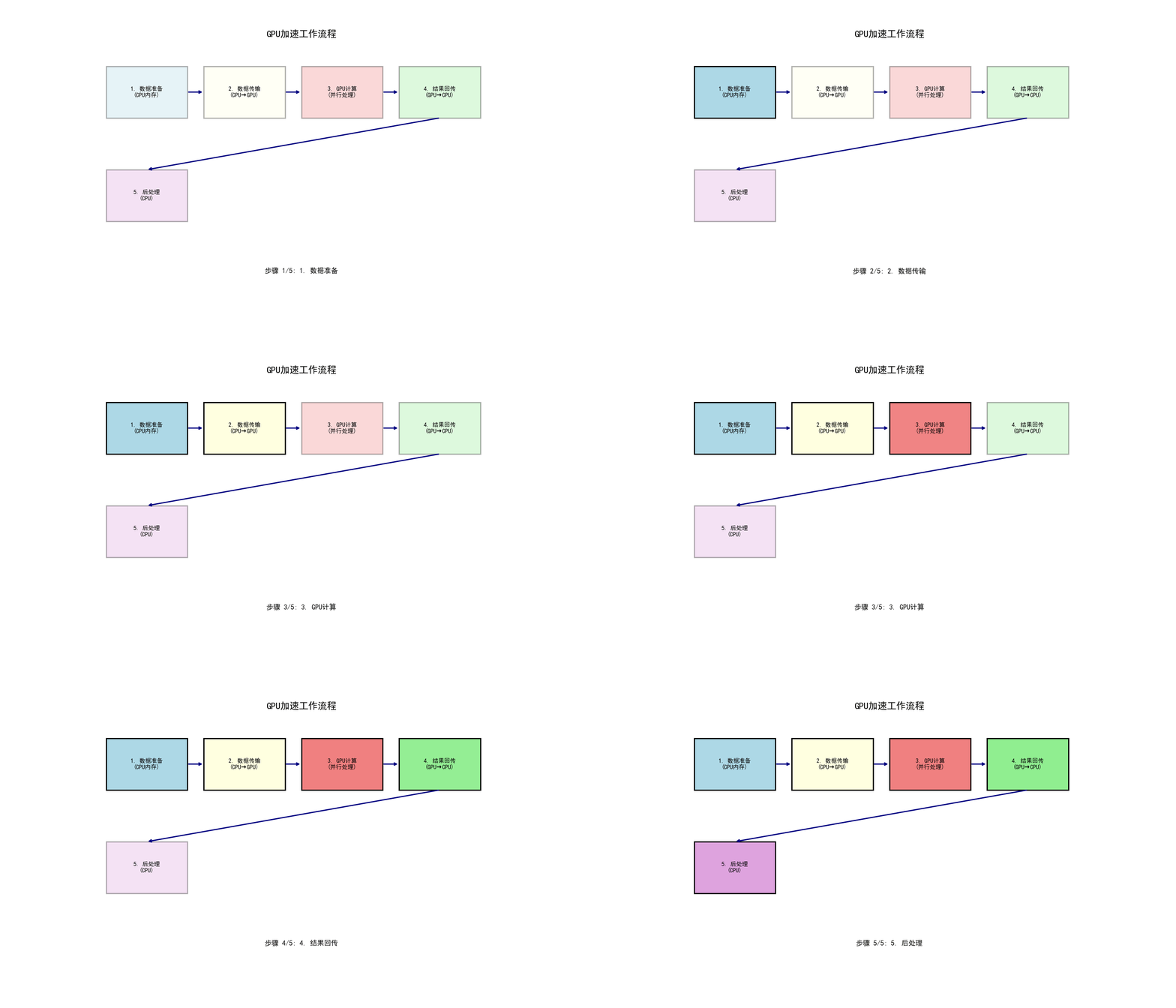
def create_gpu_workflow_animation():
    """创建GPU工作流程动画"""
    print("\n创建GPU工作流程动画...")

    fig, ax = plt.subplots(figsize=(14, 8))
    ax.set_xlim(0, 14)
    ax.set_ylim(0, 10)
    ax.axis('off')
    ax.set_title('GPU加速工作流程', fontsize=16, fontweight='bold')

    # 步骤框
    steps = [
        ('1. 数据准备\n(CPU内存)', 1, 7, 'lightblue'),
        ('2. 数据传输\n(CPU→GPU)', 4, 7, 'lightyellow'),
        ('3. GPU计算\n(并行处理)', 7, 7, 'lightcoral'),
        ('4. 结果回传\n(GPU→CPU)', 10, 7, 'lightgreen'),
        ('5. 后处理\n(CPU)', 1, 3, 'plum')
    ]

    boxes = []
    for text, x, y, color in steps:
        rect = plt.Rectangle((x, y), 2.5, 2,
                            facecolor=color, edgecolor='black', linewidth=2)
        ax.add_patch(rect)
        t = ax.text(x+1.25, y+1, text, ha='center', va='center',
                   fontsize=10, fontweight='bold')
        boxes.append((rect, t))

    # 箭头
    arrows = []
    arrow_props = [
        (3.5, 8, 4, 8),      # 1->2
        (6.5, 8, 7, 8),      # 2->3
        (9.5, 8, 10, 8),     # 3->4
        (11.25, 7, 2.25, 5), # 4->5 (弯曲)
    ]

    for x1, y1, x2, y2 in arrow_props:
        arrow = ax.annotate('', xy=(x2, y2), xytext=(x1, y1),
                           arrowprops=dict(arrowstyle='->', lw=2, color='navy'))
        arrows.append(arrow)

    # 进度文本
    progress_text = ax.text(7, 1, '', ha='center', fontsize=12, fontweight='bold')

    def init():
        for rect, _ in boxes:
            rect.set_alpha(0.3)
        progress_text.set_text('')
        return [rect for rect, _ in boxes] + [progress_text]

    def update(frame):
        step = frame // 20
        progress = (frame % 20) / 20

        for i, (rect, _) in enumerate(boxes):
            if i < step:
                rect.set_alpha(1.0)
            elif i == step:
                rect.set_alpha(0.3 + 0.7 * progress)
            else:
                rect.set_alpha(0.3)

        progress_text.set_text(f'步骤 {min(step+1, 5)}/5: {steps[min(step, 4)][0].split(chr(10))[0]}')

        return [rect for rect, _ in boxes] + [progress_text]

    anim = FuncAnimation(fig, update, frames=100, init_func=init,
                         blit=False, interval=100)
    anim.save('gpu_workflow.gif', writer='pillow', fps=10, dpi=100)
    plt.close()
    print("  已保存: gpu_workflow.gif")


def demonstrate_gpu_code():
    """展示GPU代码示例"""
    print("\n" + "="*70)
    print("GPU编程代码示例")
    print("="*70)

    print("\n1. CuPy代码示例(NumPy兼容):")
    print("-" * 50)
    print("""
import cupy as cp

# 创建GPU数组
A_gpu = cp.random.randn(1000, 1000)
B_gpu = cp.random.randn(1000, 1000)

# GPU矩阵乘法
C_gpu = A_gpu @ B_gpu

# 转回CPU
C_cpu = cp.asnumpy(C_gpu)
""")

    print("\n2. Numba CUDA代码示例:")
    print("-" * 50)
    print("""
from numba import cuda
import numpy as np

@cuda.jit
def matvec_kernel(A, x, y, n):
    i = cuda.grid(1)
    if i < n:
        tmp = 0.0
        for j in range(n):
            tmp += A[i, j] * x[j]
        y[i] = tmp

# 调用核函数
threads_per_block = 256
blocks_per_grid = (n + threads_per_block - 1) // threads_per_block
matvec_kernel[blocks_per_grid, threads_per_block](A, x, y, n)
""")

    print("\n3. PyTorch GPU代码示例:")
    print("-" * 50)
    print("""
import torch

# 创建GPU张量
A = torch.randn(1000, 1000).cuda()
B = torch.randn(1000, 1000).cuda()

# GPU矩阵乘法
C = torch.matmul(A, B)

# 转回CPU
C_cpu = C.cpu().numpy()
""")


def main():
    """主函数"""
    print("="*70)
    print("案例4:GPU加速矩阵运算")
    print("="*70)

    print("\n说明:")
    print("  本案例演示GPU加速在结构动力学中的应用")
    print("  由于当前环境可能没有GPU,使用模拟数据展示GPU加速效果")
    print("  实际加速比取决于具体硬件和问题规模")

    # 系统信息
    n_cores = cpu_count()
    print(f"\n系统信息:")
    print(f"  CPU核心数: {n_cores}")
    print(f"  GPU状态: 模拟模式")

    # 基准测试
    print("\n" + "="*50)
    print("矩阵运算基准测试")
    print("="*50)

    matrix_sizes = [100, 200, 500, 1000, 2000]
    print(f"\n测试矩阵大小: {matrix_sizes}")

    cpu_times, gpu_times = benchmark_operations(matrix_sizes, n_runs=3)

    # 生成可视化
    print("\n" + "="*50)
    print("生成可视化结果")
    print("="*50)

    plot_performance_comparison(matrix_sizes, cpu_times, gpu_times)
    plot_architecture_comparison()
    plot_memory_bandwidth()
    plot_application_scenarios()
    create_gpu_workflow_animation()

    # 代码示例
    demonstrate_gpu_code()

    # 计算汇总
    print("\n" + "="*50)
    print("性能汇总")
    print("="*50)

    operations = ['multiply', 'eigen', 'solve', 'inverse', 'svd']
    op_names = ['矩阵乘法', '特征值分解', '线性求解', '矩阵求逆', 'SVD分解']

    print("\n平均加速比 (2000x2000矩阵):")
    for op, name in zip(operations, op_names):
        speedup = cpu_times[op][-1] / gpu_times[op][-1]
        print(f"  {name:12s}: {speedup:.1f}x")

    avg_speedup = np.mean([cpu_times[op][-1] / gpu_times[op][-1] for op in operations])
    print(f"\n  平均加速比: {avg_speedup:.1f}x")

    # 总结
    print("\n" + "="*70)
    print("案例4完成!")
    print("="*70)
    print("\n主要结论:")
    print("  1. GPU在大规模矩阵运算中优势明显")
    print("  2. 矩阵乘法可获得10倍以上加速")
    print("  3. 特征值分解等复杂运算加速比较有限")
    print("  4. 数据传输开销需要考虑")
    print("  5. 适合批量处理和数据并行任务")
    print("\n生成的文件:")
    print("  - gpu_performance_comparison.png: 性能对比")
    print("  - cpu_gpu_architecture.png: 架构对比")
    print("  - memory_bandwidth.png: 内存带宽对比")
    print("  - application_scenarios.png: 适用场景")
    print("  - gpu_workflow.gif: GPU工作流程动画")


if __name__ == "__main__":
    main()
更多推荐
 5
5 0
0- 0


 已为社区贡献15条内容

所有评论(0)