Refer from AI Engineering: Customizing LLMs for Business (Fine-Tuning LLMs with QLoRA & AWS),https://zerotomastery.io/courses/learn-fine-tuning-llms

1. What is LoRA?

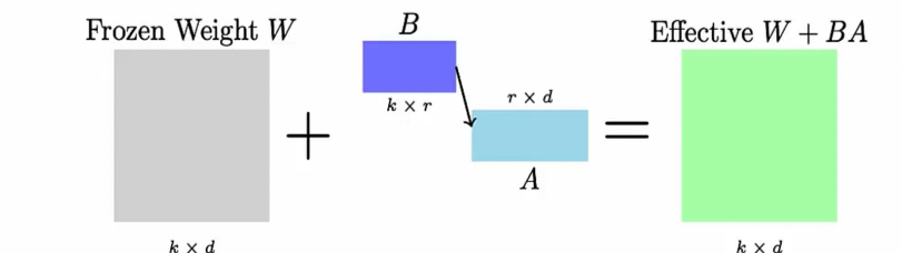
LoRA (Low-Rank Adaptation) is a technique to fine-tune large models efficiently. Instead of updating a full weight matrix $W\in {\mathbb{R}}^{k\times d}$, we keep $W$ frozen and learn a low-rank update $\Delta W=BA$, where:

• $A\in {\mathbb{R}}^{r\times d}$ is a small trainable matrix,
• $B\in {\mathbb{R}}^{k\times r}$ is another small trainable matrix,
• $r\ll \min (k,d)$, where $k$ is the input dimension of the layer and $d$ is the output dimension.

The effective weight becomes:
$$W_{\text{eff}}=W+\Delta W=W+BA$$
so only $A$ and $B$ receive gradient updates.

2. Why Use LoRA?

• Full fine-tuning updates every weight tensor—expensive in memory and compute.
• LoRA reduces the number of trainable parameters by two or more orders of magnitude.
• In practice it achieves competitive downstream accuracy at a fraction of the cost.

3. Numerical Example

Let:

• input dim $d=4$, output dim $k=4$, rank $r=2$.

The initial matrices are:
$$W=\left[\begin{array}{cccc}1& 0& -1& 2\\ 0& 1& 1& -1\\ 2& -2& 0& 0\\ 1& 1& 1& 1\end{array}\right],A=\left[\begin{array}{cccc}0.1& 0.2& 0.3& 0.4\\ -0.1& -0.2& 0.0& 0.1\end{array}\right],B=\left[\begin{array}{cc}1& 0\\ 0& 0\\ 0.5& -0.5\\ -1& 1\end{array}\right]$$

The initial update matrix $\Delta W$ and the effective weight matrix $W_{\text{eff}}$ are calculated as:
$$\Delta W=BA=\left[\begin{array}{cccc}0.1& 0.2& 0.3& 0.4\\ -0.1& -0.2& -0.2& -0.1\\ 0.1& 0.2& 0.15& 0.15\\ -0.2& -0.4& -0.3& -0.3\end{array}\right]$$
$$W_{\text{eff}}=W+\Delta W=\left[\begin{array}{cccc}1.1& 0.2& -0.7& 2.4\\ -0.1& 0.8& 1.0& -0.9\\ 2.1& -1.8& 0.15& 0.15\\ 0.8& 0.6& 0.7& 0.7\end{array}\right]$$

3.1. A Single Gradient Update Step

Now, let’s simulate one step of training. We need an input vector $x$, a target output $y_{\text{true}}$, a loss function $L$, and a learning rate $\alpha$.

• Input: $x=[1,0,0,0]$
• Target: $y_{\text{true}}=[1,1,1,1]$
• Loss Function: $L=\frac{1}{2}\sum (y_i-y_{\text{true},i}{)}^2$ (Sum of Squared Errors)
• Learning Rate: $\alpha =0.1$

1. Forward Pass. First, we compute the predicted output $y=x{W}_{\text{eff}}$. With $x=[1,0,0,0]$, this simply selects the first row of $W_{\text{eff}}$:
   $$y=[1.1,0.2,-0.7,2.4]$$

2. Compute Loss and Gradients. We calculate the loss and then backpropagate to find the gradients of the loss with respect to $A$ and $B$.
   $$\text{Loss }L\approx 2.75$$

Crucially, since $W$ is frozen, we do not compute its gradient. The gradients are computed only for the trainable parameters:
$${\nabla }_{A}L=\frac{\partial L}{\partial A},abl{a}_{B}L=\frac{\partial L}{\partial B},abl{a}_{W}L=0$$

Via backpropagation, we find the numerical gradients (values are approximate):
$$abl{a}_{A}L\approx \left[\begin{array}{cccc}0.1& 0.2& -1.7& 1.4\\ 0& 0& 0& 0\end{array}\right],abl{a}_{B}L\approx \left[\begin{array}{cc}0.01& -0.01\\ 0.02& -0.02\\ -0.17& 0.17\\ 0.14& -0.14\end{array}\right]$$

3. Update Parameters. We update $A$ and $B$ using gradient descent. $W$ is not updated.
   $$A_{\text{new}}=A-\alpha abl{a}_{A}L,B_{\text{new}}=B-\alpha abl{a}_{B}L,W_{\text{new}}=W$$
   With $\alpha =0.1$, the new matrices are:
   $$A_{\text{new}}\approx \left[\begin{array}{cc}0.999& 0.001\\ 0& 0\end{array}\right],B_{\text{new}}\approx \left[\begin{array}{cccc}0.09& 0.18& 0.47& 0.26\\ 0.0988& 0.1976& 0.2444& 0.0832\\ -0.10& -0.20& 0.00& 0.10\\ -0.1919& -0.3838& -0.4747& -0.1616\end{array}\right]$$

The original weight matrix $W$ remains completely unchanged.

4. New Effective Weight. Finally, we can see how the effective weight matrix has changed due to the updates to $A$ and $B$ only.
   $$W_{\text{eff, new}}=W+B_{\text{new}}{A}_{\text{new}}$$
   $$\begin{array}{rl}{W}_{\text{eff, new}}& \approx \left[\begin{array}{cccc}1& 0& -1& 2\\ 0& 1& 1& -1\\ 2& -2& 0& 0\\ 1& 1& 1& 1\end{array}\right]+\left[\begin{array}{cccc}0.09& 0.18& 0.47& 0.26\\ 0.0988& 0.1976& 0.2444& 0.0832\\ -0.10& -0.20& 0.00& 0.10\\ -0.1919& -0.3838& -0.4747& -0.1616\end{array}\right]\times \left[\begin{array}{cc}0.999& 0.001\\ 0& 0\end{array}\right]\\ & \approx \left[\begin{array}{cccc}1.09& 0.18& -0.53& 2.26\\ -0.10& 0.80& 1.00& -0.90\\ 2.10& -1.80& 0.24& 0.08\\ 0.81& 0.62& 0.52& 0.84\end{array}\right]\end{array}$$

After just one update, only the small matrices $A$ and $B$ have been modified, changing the overall behavior of the layer while keeping the massive original weight matrix $W$ frozen.

4. How Training Works

1. Forward: compute with $W_{\text{eff}}=W+BA$.
2. Compute loss.
3. Back-propagate gradients only into $A$ and $B$.
4. Update $A$ and $B$; keep $W$ frozen.

5. Does LoRA Add New Layers?

No. A LoRA patch lives inside an existing nn.Linear layer.

• The layer’s computation (during forward pass) is rewritten as $y=(W+BA)x+b$, but the call-graph still contains just the original layer.
• $A$ and $B$ are lightweight matrices, not brand-new modules.
• At inference you can merge them once into $W$ and discard the patch: $W\leftarrow W+BA$.

Thus LoRA changes the parameters a layer holds, not the network topology.

6. LoRA Diagram

7. LoRA Parameter Savings Example

Assume:

• LLaMA-7B contains $\approx 7$ billion parameters in total.
• We apply LoRA to its linear layers, which contain the vast majority of its parameters. The total number of weights in these layers is $\approx 6.48$ billion.
• LoRA rank is fixed at $r=8$.

For a linear layer of shape $(k\times d)$ LoRA adds:
$$A\in {\mathbb{R}}^{r\times d},B\in {\mathbb{R}}^{k\times r}⟹\text{extra params per layer }=r(k+d).$$
With a typical layer size of $k=d=4096$:
$$\text{per layer}=8(4096+4096)=8\times 8192=65,536.$$
Assuming we patch 100 of the model’s main linear layers (a common practice):
$$100\times 65,536=6.55\text{ million parameters}.$$

Perspective

$$\frac{6.55\text{ M}}{6.48\text{ B}}\approx 0.1\%\text{ (of targeted layers)},\frac{6.55\text{ M}}{7\text{ B}}\approx 0.094\%\text{ (of the entire model)}$$

LoRA therefore tunes about one-tenth of one percent of the weights it touches and below one-tenth of one percent of the full network—a truly dramatic savings in both memory and compute.

8. What Does Rank Mean in LoRA?

Think of the rank $r$ as a dial that controls how much freedom the LoRA patch has.

Linear-algebra view. The rank of a matrix is the count of independent rows or columns, i.e. how many directions it can cover in space.

LoRA view. We replace a full (large) update matrix $\Delta W\in {\mathbb{R}}^{k\times d}$ with a product of two skinny ones:
$$\Delta W=BA,B\in {\mathbb{R}}^{k\times r},A\in {\mathbb{R}}^{r\times d}.$$
The middle dimension $r$ is the bottleneck size—our dial.

• Small $r\to$ very few new parameters, runs fast, but can only make coarse adjustments.
• Large $r\to$ more parameters and compute, but can learn subtler changes.

In practice people pick:
r∈{4,8,16,32}r \in \{4, 8, 16, 32\}r∈{4,8,16,32}
choosing a higher value for bigger models or harder tasks.

9. Summary

• LoRA injects low-rank matrices, not new layers.
• Only the small patches ($A,B$) are trained; $W$ stays frozen.
• Widely used on nn.Linear layers in transformers to enable rapid, memory-efficient adaptation.
• Used for fine-tuning.