前言

泰坦尼克生存预测是机器学习经典二分类入门项目，完整覆盖数据分析、特征工程、模型训练、超参调优整套工业流程。本文基于 Python pandas、matplotlib、scikit-learn 从零搭建预测模型，对比逻辑回归与随机森林效果，附带完整代码、运行输出与可视化分析。

一、环境与数据加载

1. 导入依赖并配置可视化

import pandas as pd

import matplotlib.pyplot as plt

# 设置中文显示

plt.rcParams['font.sans-serif'] = ['SimHei']

plt.rcParams['axes.unicode_minus'] = False

# 设置 DataFrame 表格打印显示格式

pd.set_option('display.max_columns', None) # 设置最大显示列数：None代表全部列都显示

pd.set_option('display.width', 2000) # 设置输出表格宽度，数值调大，单位字符

pd.set_option('display.max_colwidth', 30) # 每列最大字符长度

# 获取泰坦尼克号数据

url = "https://raw.githubusercontent.com/datasciencedojo/datasets/master/titanic.csv"

df = pd.read_csv(url)

# 打印一些基本信息看看

print(f"数据前 5 项预览：\n{df.head()}")

print(f"\n数据集形状：", df.shape)

print(f"\n数据类型与缺失值情况：")

print(df.info())

数据前 5 项预览：

PassengerId Survived Pclass Name Sex Age SibSp Parch Ticket Fare Cabin Embarked

0 1 0 3 Braund, Mr. Owen Harris male 22.0 1 0 A/5 21171 7.2500 NaN S

1 2 1 1 Cumings, Mrs. John Bradley... female 38.0 1 0 PC 17599 71.2833 C85 C

2 3 1 3 Heikkinen, Miss. Laina female 26.0 0 0 STON/O2. 3101282 7.9250 NaN S

3 4 1 1 Futrelle, Mrs. Jacques Hea... female 35.0 1 0 113803 53.1000 C123 S

4 5 0 3 Allen, Mr. William Henry male 35.0 0 0 373450 8.0500 NaN S

数据集形状： (891, 12)

数据类型与缺失值情况：

<class 'pandas.core.frame.DataFrame'>

RangeIndex: 891 entries, 0 to 890

Data columns (total 12 columns):

# Column Non-Null Count Dtype

--- ------ -------------- -----

0 PassengerId 891 non-null int64

1 Survived 891 non-null int64

2 Pclass 891 non-null int64

3 Name 891 non-null object

4 Sex 891 non-null object

5 Age 714 non-null float64

6 SibSp 891 non-null int64

7 Parch 891 non-null int64

8 Ticket 891 non-null object

9 Fare 891 non-null float64

10 Cabin 204 non-null object

11 Embarked 889 non-null object

dtypes: float64(2), int64(5), object(5)

memory usage: 83.7+ KB

None

2. 数值统计 & 缺失值量化统计

# 数值列统计描述

print("==== 数值特征统计描述 ====")

print(df.describe())

# 统计每列缺失值数量、缺失占比

print("\n==== 缺失值统计 ====")

missing = pd.DataFrame({

"缺失数量": df.isnull().sum(),

"缺失占比(%)": round(df.isnull().sum() / len(df) *100, 2)

})

print(missing)

==== 数值特征统计描述 ====

PassengerId Survived Pclass Age SibSp Parch Fare

count 891.000000 891.000000 891.000000 714.000000 891.000000 891.000000 891.000000

mean 446.000000 0.383838 2.308642 29.699118 0.523008 0.381594 32.204208

std 257.353842 0.486592 0.836071 14.526497 1.102743 0.806057 49.693429

min 1.000000 0.000000 1.000000 0.420000 0.000000 0.000000 0.000000

25% 223.500000 0.000000 2.000000 20.125000 0.000000 0.000000 7.910400

50% 446.000000 0.000000 3.000000 28.000000 0.000000 0.000000 14.454200

75% 668.500000 1.000000 3.000000 38.000000 1.000000 0.000000 31.000000

max 891.000000 1.000000 3.000000 80.000000 8.000000 6.000000 512.329200

==== 缺失值统计 ====

缺失数量 缺失占比(%)

PassengerId 0 0.00

Survived 0 0.00

Pclass 0 0.00

Name 0 0.00

Sex 0 0.00

Age 177 19.87

SibSp 0 0.00

Parch 0 0.00

Ticket 0 0.00

Fare 0 0.00

Cabin 687 77.10

Embarked 2 0.22

二、EDA可视化：特征与生存率关系

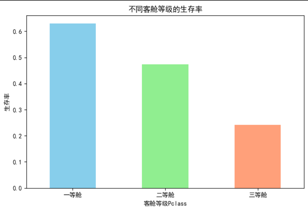
1. 客舱等级对生存率影响

plt.figure(figsize=(8, 5))

# Pclass:客舱等级 1一等，2二等，3三等

survive_pclass = df.groupby("Pclass")["Survived"].mean()

survive_pclass.plot(kind="bar", color=["#87CEEB", "#90EE90", "#FFA07A"])

plt.title("不同客舱等级的生存率")

plt.ylabel("生存率")

plt.xlabel("客舱等级Pclass")

plt.xticks([0, 1, 2], ["一等舱", "二等舱", "三等舱"], rotation=0)

plt.show()

2. 性别对生存率影响

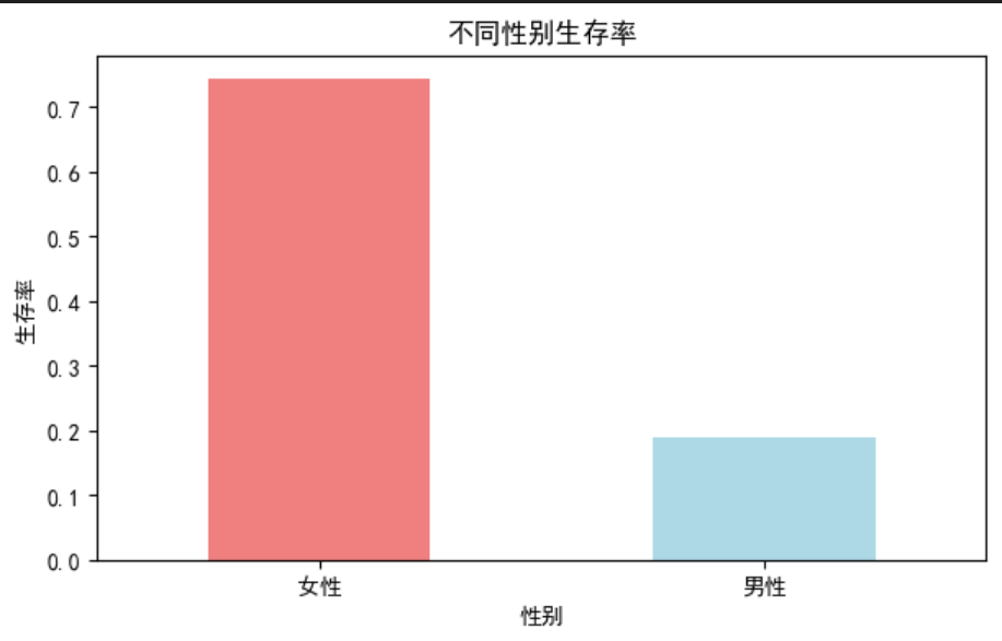
plt.figure(figsize=(7, 4))

survive_sex = df.groupby("Sex")["Survived"].mean()

survive_sex.plot(kind="bar", color=["lightcoral", "lightblue"])

plt.title("不同性别生存率")

plt.ylabel("生存率")

plt.xlabel("性别")

plt.xticks([0, 1], ["女性", "男性"], rotation=0)

plt.show()

三、特征工程：缺失值清洗+特征衍生+编码

1. 缺失值处理 & 衍生家庭人数特征

# 1. 删除Cabin列，缺失太多无利用价值

df = df.drop("Cabin", axis=1)

# 2. Age用中位数填充

df["Age"] = df["Age"].fillna(df["Age"].median())

# 3. Embarked用众数填充

df["Embarked"] = df["Embarked"].fillna(df["Embarked"].mode()[0])

# 4. 特征衍生：新增家庭大小特征 FamilySize = SibSp + Parch +1

df["FamilySize"] = df["SibSp"] + df["Parch"] + 1

# 检查处理后是否还存在缺失

print("处理完缺失后的缺失统计：")

print(df.isnull().sum())

处理完缺失后的缺失统计：

PassengerId 0

Survived 0

Pclass 0

Name 0

Sex 0

Age 0

SibSp 0

Parch 0

Ticket 0

Fare 0

Embarked 0

FamilySize 0

dtype: int64

2. 删除无用字段 + 类别特征独热编码

# 1 删除无用列

drop_cols = ["PassengerId", "Name", "Ticket"]

df = df.drop(columns=drop_cols)

# 2 One‑Hot独热编码，处理文本类别特征

df = pd.get_dummies(df, columns=["Sex", "Embarked"], drop_first=True)

print("处理完特征之后的列名：")

print(df.columns.tolist())

print("\n查看前3行数据: ")

print(df.head(3))

处理完特征之后的列名：

['Survived', 'Pclass', 'Age', 'SibSp', 'Parch', 'Fare', 'FamilySize', 'Sex_male', 'Embarked_Q', 'Embarked_S']

查看前3行数据:

Survived Pclass Age SibSp Parch Fare FamilySize Sex_male Embarked_Q Embarked_S

0 0 3 22.0 1 0 7.2500 2 True False True

1 1 1 38.0 1 0 71.2833 2 False False False

2 1 3 26.0 0 0 7.9250 1 False False True

四、数据集划分（分层抽样）

from sklearn.model_selection import train_test_split

# X：全部特征，去掉目标列 Survived

X = df.drop("Survived", axis=1)

# y：预测标签，是否存活

y = df["Survived"]

# 划分训练集、测试集

# test_size=0.2: 测试集占20%

# stratify=y: 分层抽样，保证两集合存活比例一致

X_train, X_test, y_train, y_test = train_test_split(

X, y, test_size=0.2, stratify=y, random_state=42

)

print(f"训练集大小 X_train:{X_train.shape}, y_train:{y_train.shape}")

print(f"测试集大小 X_test:{X_test.shape}, y_test:{y_test.shape}")

训练集大小 X_train:(712, 9), y_train:(712,)

测试集大小 X_test:(179, 9), y_test:(179,)

五、模型一：标准化逻辑回归

from sklearn.linear_model import LogisticRegression

from sklearn.metrics import accuracy_score, confusion_matrix, classification_report

from sklearn.preprocessing import StandardScaler

scaler = StandardScaler()

X_train_scaled = scaler.fit_transform(X_train)

X_test_scaled = scaler.transform(X_test)

lr_model = LogisticRegression(max_iter=200)

lr_model.fit(X_train_scaled, y_train)

y_pred = lr_model.predict(X_test_scaled)

print("========逻辑回归（标准化后）模型评估========")

print(f"测试集准确率 accuracy: {accuracy_score(y_test, y_pred)*100:.2f}%")

print("\n混淆矩阵：")

print(confusion_matrix(y_test, y_pred))

print("\n分类报告：")

print(classification_report(y_test, y_pred))

========逻辑回归（标准化后）模型评估========

测试集准确率 accuracy: 80.45%

混淆矩阵：

[[98 12]

[23 46]]

分类报告：

precision recall f1-score support

0 0.81 0.89 0.85 110

1 0.79 0.67 0.72 69

accuracy 0.80 179

macro avg 0.80 0.78 0.79 179

weighted avg 0.80 0.80 0.80 179

六、模型二：基础随机森林

from sklearn.ensemble import RandomForestClassifier

rf_model = RandomForestClassifier(n_estimators=100, random_state=42)

rf_model.fit(X_train, y_train)

y_pred_rf = rf_model.predict(X_test)

print("======== 随机森林模型评估 ========")

print(f"测试集准确率 accuracy: {accuracy_score(y_test, y_pred_rf)*100:.2f}%")

print("\n混淆矩阵：")

print(confusion_matrix(y_test, y_pred_rf))

print("\n分类报告：")

print(classification_report(y_test, y_pred_rf))

# 输出特征重要性

print("\n==== 特征重要性（数值越大对生存预测影响越大）====")

feature_importance = pd.DataFrame({

"feature":X_train.columns,

"importance":rf_model.feature_importances_

}).sort_values("importance", ascending=False)

print(feature_importance)

======== 随机森林模型评估 ========

测试集准确率 accuracy: 81.01%

混淆矩阵：

[[95 15]

[19 50]]

分类报告：

precision recall f1-score support

0 0.83 0.86 0.85 110

1 0.77 0.72 0.75 69

accuracy 0.81 179

macro avg 0.80 0.79 0.80 179

weighted avg 0.81 0.81 0.81 179

==== 特征重要性（数值越大对生存预测影响越大）====

feature importance

4 Fare 0.273412

6 Sex_male 0.261490

1 Age 0.237682

0 Pclass 0.085662

5 FamilySize 0.050495

2 SibSp 0.033592

3 Parch 0.024457

8 Embarked_S 0.024002

7 Embarked_Q 0.009208

导出测试集预测结果

# 获取测试集预测结果

test_result = X_test.copy()

test_result["真实_Survived"] = y_test

test_result["预测_Survived"] = y_pred_rf

# 输出csv文件，保存到你当前VSCode工作目录

test_result.to_csv("1.titanic_test_predict.csv", index=False, encoding="utf_8_sig")

print("1.预测文件已保存：titanic_test_predict.csv")

七、超参调优：网格搜索GridSearchCV优化随机森林

from sklearn.model_selection import GridSearchCV

# 1、设置要搜索的参数字典

param_grid = {

"n_estimators": [50, 100, 150], # 森林中决策树棵数

"max_depth": [3, 5, 7, 9, 11] # 树最大深度，重点！

}

# 2、基础随机森林模型

rf = RandomForestClassifier(random_state=42)

# 3、网格搜索，5折交叉验证

grid_search = GridSearchCV(

estimator=rf,

param_grid=param_grid,

cv=5, # 5折交叉验证

scoring="accuracy", # 评估指标用准确率

n_jobs=-1 # n_jobs=-1 使用电脑全部CPU，加速搜索

)

# ⚠️注意：fit只用训练集！绝对不能把X_test放进来！

grid_search.fit(X_train, y_train)

# 输出最优参数、最优交叉验证得分

print("✅网格搜索得到的最优参数：")

print(grid_search.best_params_)

print(f"\n训练集上5折交叉验证最优准确率：{grid_search.best_score_*100:.2f}%")

# 获取调参完毕的最优模型

best_rf = grid_search.best_estimator_

# 使用最优模型，在【从未见过的测试集】上评估！

y_pred_best = best_rf.predict(X_test)

print("\n======== 调参后最优模型，测试集评估 ========")

print(f"测试集准确率：{accuracy_score(y_test, y_pred_best)*100:.2f}%")

print(classification_report(y_test, y_pred_best))

feature_importance = pd.DataFrame({

"feature":X_train.columns,

"importance":best_rf.feature_importances_

}).sort_values("importance", ascending=False)

print("\n调参后特征重要性：")

print(feature_importance)

✅网格搜索得到的最优参数：

{'max_depth': 3, 'n_estimators': 100}

训练集上5折交叉验证最优准确率：82.17%

======== 调参后最优模型，测试集评估 ========

测试集准确率：79.89%

precision recall f1-score support

0 0.78 0.94 0.85 110

1 0.85 0.58 0.69 69

accuracy 0.80 179

macro avg 0.82 0.76 0.77 179

weighted avg 0.81 0.80 0.79 179

调参后特征重要性：

feature importance

6 Sex_male 0.451692

4 Fare 0.177798

0 Pclass 0.161332

1 Age 0.074909

5 FamilySize 0.060430

2 SibSp 0.031093

8 Embarked_S 0.022414

3 Parch 0.012901

7 Embarked_Q 0.007431

八、项目总结与优化思路

1. 实验结论

1. 数据规律：性别、舱位票价、年龄是决定生存的三大核心特征，女性、一等舱乘客存活概率更高；
2. 模型对比：基础随机森林(81.01%)效果略优于标准化逻辑回归(80.45%)；
3. 调参效果：网格搜索仅提升训练集交叉验证精度，测试集准确率小幅下跌，出现轻微过拟合；限制树深度后性别特征区分权重大幅提升。

2. 后续优化方向

1. 深度特征挖掘：从 Name 字段提取 Mr/Mrs/Miss 头衔，新增儿童/成人年龄分箱特征；
2. 算法升级：尝试 XGBoost、LightGBM、SVM 等模型，搭配正则缓解过拟合；
3. 工程优化：增加特征筛选、归一化对比、学习曲线绘制，直观观测过拟合程度；
4. 评价指标补充：除准确率外，重点关注存活样本召回率，贴合项目业务场景。

九、最后再唠唠

由于我做的时候使用的是 Jupyter Notebook，所以代码都是一段一段的不好看，还请见谅！此外如果聪明的你发现了代码和表述有错误或者有更好的提议，还请告知，谢谢！