前言

本篇文章记录 MIT S.184 作业 Lab 3: Diffusion Transformer and VAEs 的实现，和大家一起分享交流😄。

reference：https://github.com/eje24/iap-diffusion-labs

Part 3: Building a Diffusion Transformer

到目前为止，我们已经讨论了 classifier-free guidance，以及在模型设计和模型训练中必须考虑的一些问题。接下来剩下的，就是具体讨论模型的选择。

特别地，我们平时常用的 MLP，虽然对于前一个 lab 中的简单分布来说已经足够，但对于现在的图像任务来说已经不够了。

为此，我们将逐个组件实现一个 diffusion transformer！

Question 3.1: Fourier Time Encoder

首先，我们实现一个 Fourier time encoder，它会将一个标量时间值 $t\in [0,1]$ 映射为：

$$t^{\text{emb}}={\left[\begin{array}{cccccc}\cos (2\pi w_{1}t)& \cdots & \cos (2\pi w_{d}t)& \sin (2\pi w_{1}t)& \cdots & \sin (2\pi w_{d}t)\end{array}\right]}^T,$$

其中权重 $w_i\sim \mathcal{N}(0,1)$ 从标准正态分布中采样得到。

Your job：实现 FourierEncoder。

class FourierEncoder(nn.Module):
    """
    Based on https://github.com/lucidrains/denoising-diffusion-pytorch/blob/main/denoising_diffusion_pytorch/karras_unet.py#L183
    """
    def __init__(self, dim: int):
        super().__init__()
        assert dim % 2 == 0
        self.half_dim = dim // 2
        self.weights = nn.Parameter(torch.randn(1, self.half_dim))

    def forward(self, t: torch.Tensor) -> torch.Tensor:
        """
        Args:
        - t: b
        Returns:
        - embeddings: b d
        """
        # Step 1: compute frequencies f_i = 2 * pi * w_i * t
        t = t.view(-1, 1)
        freqs = 2 * math.pi * t * self.weights

        # Step 2: compute sin(f_i) and cos(f_i)
        cos_emb = torch.cos(freqs)
        sin_emb = torch.sin(freqs)

        # Step 3: Concatenate and return
        embeddings = torch.cat([cos_emb, sin_emb], dim=-1)
        return embeddings

这个 FourierEncoder 的作用是把一维时间标量 $t$ 映射成高维时间 embedding。

在 diffusion / flow matching 模型中，神经网络必须知道当前处于哪个时间步。比如：

• $t$ 接近 0：输入更像噪声
• $t$ 接近 1：输入更像真实图像

如果只把一个标量 $t$ 直接输入模型，表达能力比较弱。因此这里用 Fourier 特征把时间映射到更高维空间。

1. 处理时间形状

t = t.view(-1, 1)

输入 t 的形状是 (batch_size,)，为了和 self.weights 相乘，需要把它变成 (batch_size, 1)，这样通过广播可以得到 (batch_size, half_dim)。

2. 计算 Fourier 频率

freqs = 2 * math.pi * t * self.weights

这一行对应公式中的：

$$f_t=2\pi w_{i}t$$

其中：

• t 的形状是 (b, 1)；
• self.weights 的形状是 (1, half_dim)；
• freqs 的形状是 (b, half_dim)。

也就是说，对于 batch 中每个时间 t，都会计算一组不同频率下的相位。

3. 计算 cos 和 sin 特征

cos_emb = torch.cos(freqs)
sin_emb = torch.sin(freqs)

对应 $\cos (2\pi w_{i}t)$ 和 $\sin (2\pi w_{i}t)$ ，这两组特征能够让模型更容易表达关于时间的周期性、高频和低频变化。

4. 拼接得到最终 embedding

embeddings = torch.cat([cos_emb, sin_emb], dim=-1)

拼接后形状为 (batch_size, dim)，这正对应：

$$t^{\text{emb}}={\left[\begin{array}{cccccc}\cos (2\pi w_{1}t)& \cdots & \cos (2\pi w_{d}t)& \sin (2\pi w_{1}t)& \cdots & \sin (2\pi w_{d}t)\end{array}\right]}^T,$$

Question 3.2: Patchifier

Patchifier 接收一个图像张量，形状为 b c 32 32，然后将其 patchify，也就是切成 patch，并转换为形状 b (h / p * w / p) d，其中：

• d 表示 Diffusion Transformer 的 hidden dimension，也就是下面实现中的 dim；
• p 表示 patch size；
• h 和 w 分别表示图像高度和宽度。

这个过程分成两步：

1. 使用一个卷积层，将输入从 b c 32 32 映射到 b d h/p w/p
2. 将张量从 b d h/p w/p 重排成 b (h/p w/p) d，也就是说，一张图像会被转换成 n = h/p * w/p 个 token，每个 token 的维度是 d。

注意，对于本节中训练的标准 pixel-space diffusion transformer 来说，c=1，因为 MNIST 是单通道灰度图。但是在第 5 节训练 latent diffusion transformer 时，情况将不再是这样。

Your job：实现 Patchifier。

class Patchifier(nn.Module):
  def __init__(self, img_size: int, patch_size: int, c_in: int, dim: int):
    super().__init__()
    assert img_size % patch_size == 0, "Image size must be divisible by patch size"

    self.img_size = img_size
    self.patch_size = patch_size
    self.c_in = c_in
    self.dim = dim
    self.num_patches = (img_size // patch_size) ** 2

    self.proj = nn.Conv2d(
        in_channels=c_in,
        out_channels=dim,
        kernel_size=patch_size,
        stride=patch_size
    )
    self.rearrange = Rearrange('b c h w -> b (h w) c')


  def forward(self, x: torch.Tensor) -> torch.Tensor:
    """
    Args:
    - x: (bs, 1, img_size, img_size)
    Returns:
    - x: (bs, 1, img_size, img_size)
    """
    x = self.proj(x)
    x = self.rearrange(x)
    return x

Patchifier 的作用是把图像转换成 Transformer 可以处理的 token 序列。

Transformer 原本处理的是序列，例如 NLP 中的词 token。对于图像，我们需要先把二维图像切成多个 patch，再把每个 patch 映射成一个 token embedding。

1. 初始化参数

def __init__(self, img_size: int, patch_size: int, c_in: int, dim: int):

这里几个参数含义是：

• img_size：图像大小，例如 MNIST resize 后是 32
• patch_size：每个 patch 的边长
• c_in：输入通道数，例如 MNIST 是 1
• dim：Transformer hidden dimension，也就是每个 patch token 的维度

例如：

img_size = 32
patch_size = 4
c_in = 1
dim = 128

那么一张图像会被切成：

$$\frac{32}{4}\times \frac{32}{4}=8\times 8=64$$

个 patch，每个 patch 被映射成一个 128 维 token。

2. 计算 patch 数量

self.num_patches = (img_size // patch_size) ** 2

因为这里默认图像高度和宽度都等于 img_size，所以 patch 总数为：

$$n=\frac{h}{p}\times \frac{w}{p}$$

3. 使用卷积实现 patch embedding

self.proj = nn.Conv2d(
    in_channels=c_in,
    out_channels=dim,
    kernel_size=patch_size,
    stride=patch_size
)

这是整个 Patchifier 的关键。

它使用一个卷积层将图像从 (bs, c_in, img_size, img_size) 变成 (bs, dim, img_size / patch_size, img_size / patch_size)，这里我们设置：

kernel_size = patch_size
stride = patch_size

这意味着卷积核每次正好覆盖一个 patch，并且移动步长也是一个 patch 的大小。因此不同 patch 之间不会重叠。

4. 重排成 token 序列

self.rearrange = Rearrange("b d h w -> b (h w) d")

卷积输出是 b d h' w'，其中：

$$h^{\prime }=h/p,w^{\prime }=w/p.$$

Transformer 需要的是 token 序列形式 b n d，所以需要把空间维度 h' 和 w' 合并成 token 数量：

$$n=h^{\prime }{w}^{\prime }=\frac{h}{p}\frac{w}{p}.$$

Question 3.3: Diffusion Transformer

现在，我们的数据形状是 b n d，其中 n 表示每张图像对应的 image tokens 数量。接下来，我们会将这些 tokens 输入到 Transformer 中。

本着 “硬着头皮把墙撞穿” 的精神，你将实现整个 Transformer！特别是，如果你之前还没有从头实现过 attention，那么从头实现 attention 是一个非常有价值的练习。

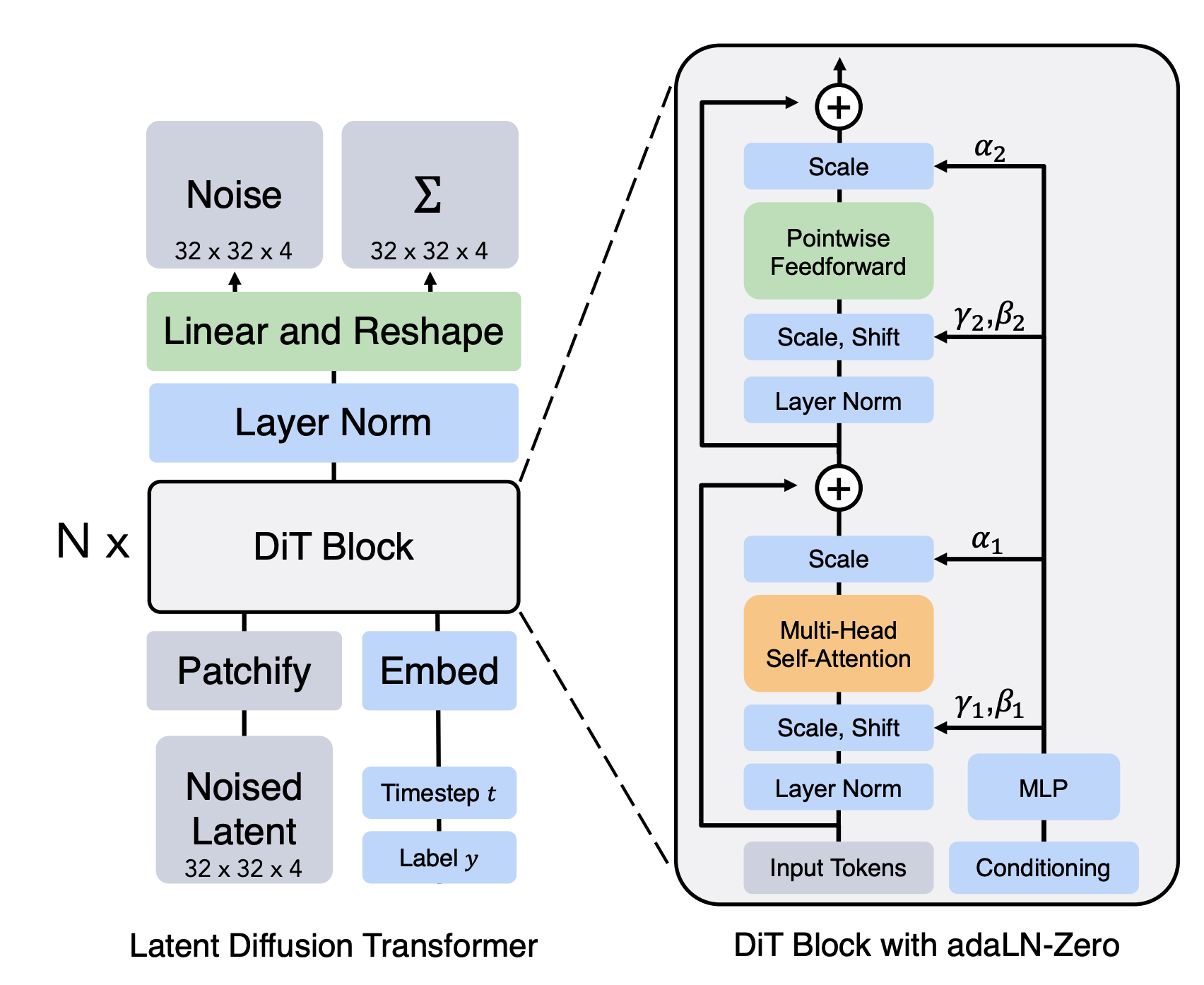
在完成这一题时，可以参考上面的 diffusion transformer 架构图，该图来自文献 [William+ 2023]。

Your job：完成 MHA，也就是 multi-headed self-attention，DiffusionTransformerLayer，以及 DiffusionTransformer。

Recommended steps：我们从外到内逐步完成。

1. 首先，实现 DiffusionTransformer。特别地，我们推荐使用固定的、每个位置对应的可学习位置编码，例如：

nn.Parameter(torch.randn(n_tokens, dim))

注意，你可以通过参数 n_tokens 得到固定的 token 数量。此外，你还需要初始化 depth 个 DiffusionTransformerLayer 实例。然后，前向传播只需要将位置编码加到输入 token 上，注意广播，然后依次通过 diffusion transformer layers。

2. 第二，实现 DiffusionTransformerLayer。这里可以参考上面的结构图。注意，adaLN-Zero 指的是将 conditioning MLP 的权重初始化为 0，通常只需要把最后一层初始化为 0 即可。虽然这一步是可选的，但将这些残差连接初始化为 0 通常有助于稳定训练。

我们注意到， $\gamma ,\beta ,\alpha$ 的形状应该是 b d，注意广播。scale 和 shift 操作通常实现为：

$$x\mapsto x\ast (1+\gamma )+\beta$$

对于 feed-forward network，可以使用前面定义的 MLP 类。DiT 中一个典型选择是使用 hidden dimensions [dim, 4 * dim, dim]。

3. 最后，实现 multi-headed self-attention。

OK，我们按照作业中建议的步骤从外到内来实现。

先看 DiffusionTransformer 的实现：

class DiffusionTransformer(nn.Module):
  def __init__(
      self,
      depth: int,
      n_tokens: int,
      dim: int,
      **layer_kwargs,
  ):
    """
    Args:
    - n_tokens: sequence length (for sake of positional embeddings)
    - dim: dimension of hidden layers
    - heads: number of attention heads
    - depth: number of layers
    """
    super().__init__()

    self.n_tokens = n_tokens
    self.dim = dim

    self.pos_embedding = nn.Parameter(torch.randn(n_tokens, dim) * 0.02)
    
    self.layers = nn.ModuleList([
        DiffusionTransformerLayer(dim=dim, **layer_kwargs)
        for _ in range(depth)
    ])


  def forward(self, x: torch.Tensor, c: torch.Tensor) -> torch.Tensor:
    """
    Args:
    - x: b n d
    - c: b d
    Returns:
    - x: b n d
    """
    x = x + self.pos_embedding.unsqueeze(0)

    for layer in self.layers:
        x = layer(x, c)

    return x

DiffusionTransformer 是多个 DiffusionTransformerLayer 的堆叠。

1. 位置编码

self.pos_embedding = nn.Parameter(torch.randn(n_tokens, dim) * 0.02)

Transformer 本身对 token 顺序不敏感，因此必须加入位置编码，让模型知道每个 patch token 来自图像中的哪个位置。

这里使用的是可学习位置编码，形状为 n_tokens d，前向传播中：

x = x + self.pos_embedding.unsqueeze(0)

将其广播到 batch 维 1 n d，然后加到所有样本的 token 上。

2. 堆叠 Transformer Layers

self.layers = nn.ModuleList([
    DiffusionTransformerLayer(dim=dim, **layer_kwargs)
    for _ in range(depth)
])

这里创建 depth 个 DiT block。例如 depth = 6 就表示主干网络中有 6 层 DiT block。

3. 前向传播

for layer in self.layers:
    x = layer(x, c)

每一层都接收 x: b n d 和 c: b d，其中 c 是 conditioning embedding，后面一般由时间 embedding 和类别 embedding 融合得到。最终输出仍然是 b n d，也就是每个 token 的 hidden representation。

接着看 DiffusionTransformerLayer 的实现，我们参考上面的结构图来实现：

class DiffusionTransformerLayer(nn.Module):
  def __init__(
      self,
      dim: int,
      heads: int,
  ):
    """
    Args:
    - n_tokens: sequence length (for sake of positional embeddings)
    - dim: dimension of hidden layers
    - heads: number of attention heads
    """
    super().__init__()

    # Init normalization
    self.attn_norm = nn.LayerNorm(dim)
    self.ff_norm = nn.LayerNorm(dim)

    # Initialize conditioning to zero - stabilizes residual connection!
    self.conditioning_mlp = MLP([dim, 4 * dim, 6 * dim], final_init=True)

    # Init attention
    self.attn = MHA(dim=dim, heads=heads)

    # Init feedforward
    self.ff = MLP([dim, 4 * dim, dim])

  def forward(self, x: torch.Tensor, c: torch.Tensor) -> torch.Tensor:
    """
    Args:
    - x: b n d
    - c: b d
    Returns:
    - x: b n d
    """
    # Compute conditioning gating, scaling, and bias
    alpha1, gamma1, beta1, alpha2, gamma2, beta2 = self.conditioning_mlp(c).chunk(6, dim=-1)

    alpha1 = alpha1.unsqueeze(1)
    gamma1 = gamma1.unsqueeze(1)
    beta1 = beta1.unsqueeze(1)

    alpha2 = alpha2.unsqueeze(1)
    gamma2 = gamma2.unsqueeze(1)
    beta2 = beta2.unsqueeze(1)

    # Attention + residual connection
    h = self.attn_norm(x)
    h = h * (1 + gamma1) + beta1
    h = self.attn(h)
    x = x + alpha1 * h

    # Feedforward + residual connection
    h = self.ff_norm(x)
    h = h * (1 + gamma2) + beta2
    h = self.ff(h)
    x = x + alpha2 * h

    return x

DiffusionTransformerLayer 对应图中的一个 DiT Block with adaLN-Zero。

它主要由两条残差分支组成：

• LayerNorm + adaLN modulation + MHA + gated residual
• LayerNorm + adaLN modulation + FFN + gated residual

其中 conditioning 变量 c 会控制每个 block 中的 scale、shift 和 residual gate。

1. LayerNorm

self.attn_norm = nn.LayerNorm(dim)
self.ff_norm = nn.LayerNorm(dim)

Transformer 中通常会在 attention 和 feed-forward 前做 LayerNorm。

这里采用的是 pre-norm 结构：

• Norm -> Attention -> Residual
• Norm -> FFN -> Residual

2. Conditioning MLP

self.conditioning_mlp = MLP([dim, 4 * dim, 6 * dim], final_init=True)

这个 MLP 接收 conditioning 向量 c: b d，输出 6 组参数 alpha1, gamma1, beta1, alpha2, gamma2, beta2，每组形状都是 b d，它们分别用于 attention 分支和 feed-forward 分支：

• attention 分支：gamma1, beta1, alpha1
• feed-forward 分支：gamma2, beta2, alpha2

其中：

• $\gamma$：scale 参数；
• $\beta$：shift 参数；
• $\alpha$：residual gate 参数。

final_init=True 会把 conditioning MLP 的最后一层初始化为 0。这样一开始：

alpha ≈ 0
gamma ≈ 0
beta ≈ 0

所以 DiT block 初始时更接近 identity mapping，有助于训练稳定。这就是 adaLN-Zero 的思想。

3. Attention 分支

h = self.attn_norm(x)
h = h * (1 + gamma1) + beta1
h = self.attn(h)
x = x + alpha1 * h

它对应：

$$h=\text{LayerNorm}(x)$$

然后使用 conditioning 参数调制：

$$h\leftarrow h\cdot (1+{\gamma }_1)+{\beta }_1.$$

接着通过 self-attention：

$$h\leftarrow \text{MHA}(h)$$

最后通过 residual gate 加回原输入：

$$x\leftarrow x+{\alpha }_{1}h$$

这里 alpha1 也是由 conditioning MLP 生成的，因此模型可以根据时间和类别条件控制 residual 分支的强度。

4. Feed-Forward 分支

h = self.ff_norm(x)
h = h * (1 + gamma2) + beta2
h = self.ff(h)
x = x + alpha2 * h

这部分结构与 attention 分支类似，只是中间模块换成了前馈网络：

$$\text{MLP}:d\to 4d\to d$$

它主要用于对每个 token 独立做非线性变换，而 attention 则负责 token 之间的信息交互。

最后，我们来看 multi-headed self-attention 的实现：

class MHA(nn.Module):
  """
  Multi-headed self-attention
  """
  def __init__(self, dim: int, heads: int):
    super().__init__()
    assert dim % heads == 0

    self.dim = dim
    self.heads = heads
    self.head_dim = dim // heads

    self.to_qkv = nn.Linear(dim, dim * 3)
    self.to_out = nn.Linear(dim, dim)


  def forward(self, x: torch.Tensor) -> torch.Tensor:
    """
    Args:
    - x: b n d
    Returns:
    - x: b n d
    """
    b, n, d = x.shape

    # Compute queries, keys, and values
    q, k, v = self.to_qkv(x).chunk(3, dim=-1)  # b n d

    # Fold head into batch dimension
    q = rearrange(q, "b n (h dh) -> (b h) n dh", h=self.heads)
    k = rearrange(k, "b n (h dh) -> (b h) n dh", h=self.heads)
    v = rearrange(v, "b n (h dh) -> (b h) n dh", h=self.heads)

    # Compute attention
    attn_logits = torch.bmm(q, k.transpose(1, 2)) / math.sqrt(self.head_dim)  # (b h) n n
    attn = torch.softmax(attn_logits, dim=-1)

    # Combine with values
    out = torch.bmm(attn, v)  # (b h) n dh

    # Unfold heads
    out = rearrange(out, "(b h) n dh -> b n (h dh)", h=self.heads, b=b)

    # Pass throuh FF and return
    out = self.to_out(out)
    return out

MHA 的输入是 x: b n d 也就是一批 token 序列。Self-attention 的核心思想是：每个 token 都可以根据与其他 token 的相关性，从所有 token 中聚合信息。

1. 初始化

self.heads = heads
self.head_dim = dim // heads
self.to_qkv = nn.Linear(dim, 3 * dim)
self.to_out = nn.Linear(dim, dim)

这里 dim 会被拆成多个 attention heads：

$$d=h\cdot d_h$$

其中：

• $h$ 是 head 数量；
• $d_h$ 是每个 head 维度。

to_qkv 一次性生成 query、key、value：

$$Q,K,V$$

因此输出维度是 3 * dim。

2. 计算 Q、K、V

q, k, v = self.to_qkv(x).chunk(3, dim=-1)

这一步将 b n d 映射为三个张量：

q: b n d
k: b n d
v: b n d

3. 拆分多头

q = rearrange(q, "b n (h dh) -> (b h) n dh", h=self.heads)

这里把 head 维度折叠进 batch 维度，得到：

q: (b * heads) n head_dim

k 和 v 同理。

这样后面可以直接使用 torch.bmm 做 batch matrix multiplication。

4. 计算 attention 权重

attn_logits = torch.bmm(q, k.transpose(1, 2)) / math.sqrt(self.head_dim)
attn = torch.softmax(attn_logits, dim=-1)

这对应标准 scaled dot-product attention：

$$\text{Attention}(Q,K,V)=\text{softmax}(\frac{Q{K}^T}{\sqrt{d_h}})V.$$

其中除以 $\sqrt{d_h}$ 是为了避免 dot product 数值过大，导致 softmax 过于尖锐。

5. 聚合 Value

out = torch.bmm(attn, v)

这一步让每个 token 根据 attention 权重，从所有 token 的 value 中加权汇聚信息。输出形状仍然是 (b * heads) n head_dim。

6. 合并多头

out = rearrange(out, "(b h) n dh -> b n (h dh)", h=self.heads, b=b)

将多头结果重新拼回 b n d，最后经过输出投影：

out = self.to_out(out)

得到最终 attention 输出。

OK，以上就是 Diffusion Transformer 的完整实现。

Question 3.4 Depatchifier

在经过 diffusion transformer 之后，我们需要将张量从 b n d 转换回 b 1 h w。

Your job：实现 Depatchifier。

Hints：一种实现方式如下：

1. 先做某种归一化，例如 nn.LayerNorm 或 nn.RMSNorm 都可以；
2. 通过某个 MLP，将张量变成 b (h/p w/p) (f p p)，也就是说，对于 patch size 为 $p$ 、最终中间通道数为 $f$ ，把最后一维映射到 $f{p}^2$ ；
3. 将其重排成 b f h w；
4. 再通过最后一个卷积层，得到形状为 b 1 h w 的输出。

class Depatchifier(nn.Module):
  def __init__(self, img_size: int, patch_size: int, dim: int, final_dim: int, c_out: int):
    super().__init__()
    self.patch_size = patch_size
    assert img_size % patch_size == 0, "Image size must be divisible by patch size"

    self.img_size = img_size
    self.num_patches_per_side = img_size // patch_size
    self.final_dim = final_dim
    self.c_out = c_out

    self.norm = nn.LayerNorm(dim)

    self.mlp = MLP([
        dim,
        final_dim * patch_size * patch_size
    ])

    self.rearrange = Rearrange(
        "b (h w) (f p1 p2) -> b f (h p1) (w p2)",
        h=self.num_patches_per_side,
        w=self.num_patches_per_side,
        p1=patch_size,
        p2=patch_size,
        f=final_dim,
    )

    self.final_conv = nn.Conv2d(
        in_channels=final_dim,
        out_channels=c_out,
        kernel_size=3,
        padding=1
    )


  def forward(self, x: torch.Tensor) -> torch.Tensor:
    """
    Args:
    - x: b n d
    Returns:
    - x: b 1 32 32
    """
    x = self.norm(x)
    x = self.mlp(x)
    x = self.rearrange(x)
    x = self.final_conv(x)
    return x

Depatchifier 的作用是把 Transformer 输出的 token 序列重新变回图像。前面 Patchifier 做的是：

$$(b,c,h,w)\to (b,n,d)$$

而这里做的是反方向：

$$(b,n,d)\to (b,c_{\text{out}},h,w)$$

1. 初始化基本参数

self.patch_size = patch_size
self.img_size = img_size
self.num_patches_per_side = img_size // patch_size

2. LayerNorm

self.norm = nn.LayerNorm(dim)

Transformer 输出的每个 token 维度是 dim，所以这里对最后一维做归一化。输入形状 b n d，归一化后仍然是 b n d，这一步可以稳定后续 projection。

3. MLP 投影

self.mlp = MLP([
    dim,
    final_dim * patch_size * patch_size
])

每个 token 原本是 dim 维，现在要把它映射成一个小 patch。对于每个 patch，我们希望它最终能对应一个形状为 final_dim × patch_size × patch_size 的小块。因此每个 token 需要被映射到 $\text{find\_dim}\times {\text{patch\_size}}^2$ 维。

4. Rearrange 重排回图像网格

self.rearrange = Rearrange(
    "b (h w) (f p1 p2) -> b f (h p1) (w p2)",
    h=self.num_patches_per_side,
    w=self.num_patches_per_side,
    p1=patch_size,
    p2=patch_size,
    f=final_dim,
)

这一步是 Depatchifier 的核心，它把 token 序列重新摆回二维图像网格。

输入：

b (h w) (f p1 p2)

其中：

• h w 是 patch 网格数量；
• f 是中间特征通道数；
• p1 p2 是每个 patch 的空间大小。

输出：

b f (h p1) (w p2)

也就是把所有 patch 拼回一张完整图像。

5. 最后一层卷积

self.final_conv = nn.Conv2d(
    in_channels=final_dim,
    out_channels=c_out,
    kernel_size=3,
    padding=1
)

重排后的张量形状是 b final_dim img_size img_size，但我们最终需要输出图像形状 b c_out img_size img_size。对于 MNIST，通常 c_out = 1，所以最后通过一个 $3\times 3$ 卷积，将中间通道数 final_dim 映射到目标输出通道数 c_out。

Question 3.5: Putting It All Together

最后，让我们使用 DiffusionTransformerFlowModel 类，实现一个基于 DiT 的 guided flow model $u_t^{\theta }(x|y)$ 。

Your job：实现 DiffusionTransformerFlowModel。

Hints：

1. 为了嵌入 guiding input y，你需要使用类别标签。可以复用你在 MLPConditionalVectorField 中的实现。特别地，我们推荐使用 nn.Embedding(num_classes=11, embedding_dim=dim)，注意这里使用的是 11 类，而不是 10 类，因为还需要额外包含 null label。
2. 按照 DiT 总览图来实现：先分别嵌入 $t$ 和 $y$ ，然后将它们相加得到 guiding variable。将 $x$ 输入 patchifier，然后将 patchifier 的输出和 $t+y$ 输入 diffusion transformer。最后，将 DiT 输出传入 depatchifier。

class DiffusionTransformerFlowModel(ConditionalVectorField):
  def __init__(
      self,
      img_size: int = 32,
      patch_size: int = 8,
      num_layers: int = 12,
      c: int = 1,
      dim: int = 256,
      heads: int = 4,
      final_dim: int = 10,
      n_classes: int = 11,
    ):
      super().__init__()
      # 0. Construct time_embedder and y_embedder
      self.time_embedder = FourierEncoder(dim)
      self.y_embedder = nn.Embedding(n_classes, dim)

      # 1. Construct patchifier
      self.patchifier = Patchifier(
          img_size=img_size,
          patch_size=patch_size,
          c_in=c,
          dim=dim
      )

      # 2. Construct DiT
      n_tokens = (img_size // patch_size) ** 2
      self.dit = DiffusionTransformer(
          depth=num_layers,
          n_tokens=n_tokens,
          dim=dim,
          heads=heads
      )

      # 3. Construct de-patchifier
      self.depatchifier = Depatchifier(
          img_size=img_size,
          patch_size=patch_size,
          dim=dim,
          final_dim=final_dim,
          c_out=c
      )

  def forward(self, x: torch.Tensor, t: torch.Tensor, y: torch.Tensor) -> torch.Tensor:
    """
    Args:
    - x: b 1 32 32
    - t: b 1 1 1
    - c: b 1 1 1
    Returns:
    - u_t^theta(x|y): b 1 32 32
    """
    # 1. Embed time and y
    t = t.view(t.shape[0])
    t_emb = self.time_embedder(t)
    y_emb = self.y_embedder(y.long())
    c = t_emb + y_emb

    # 2. Patchify
    x = self.patchifier(x)

    # 3. Pass through DiT
    x = self.dit(x, c)

    # 4. Depatchify
    x = self.depatchifier(x)

    return x

这个类就是完整的条件向量场模型 $u_t^{\theta }(x|y)$ ，它接收当前 noisy image $x$ 、时间 $t$ 、类别标签 $y$ ，输出一个和图像同形状的向量场，用于 Flow Matching / ODE 采样。

1. 时间嵌入器

self.time_embedder = FourierEncoder(dim)

FourierEncoder 将时间标量 $t$ 映射成 dim 维向量：

$$t\to t^{emb}\in {\mathbb{R}}^d$$

这样模型就能知道当前处于生成路径的哪个阶段。

2. 类别嵌入器

self.y_embedder = nn.Embedding(n_classes, dim)

这里将离散标签 $y$ 映射成 dim 维向量：

$$y\to y^{emb}\in {\mathbb{R}}^d$$

对于 MNIST，真实标签是 0~9，而 CFG 还需要一个 null label，所以总类别数是 11。

3. 条件向量 $c$

在 forward 中：

t = t.view(t.shape[0])
t_emb = self.time_embedder(t)
y_emb = self.y_embedder(y.long())
c = t_emb + y_emb

这里把时间嵌入和类别嵌入相加，得到 conditioning vector：

$$c=t^{emb}+y^{emb}$$

其形状是 (batch_size, dim)，这个 c 会传入每一个 DiT block，用于 adaLN-Zero 条件调制。

4. Patchifier

self.patchifier = Patchifier(
    img_size=img_size,
    patch_size=patch_size,
    c_in=c,
    dim=dim
)

Patchifier 将图像从 b c h w 转换成 Transformer token 序列 b n d。

5. Diffusion Transformer

self.dit = DiffusionTransformer(
    depth=num_layers,
    n_tokens=n_tokens,
    dim=dim,
    heads=heads
)

这里构造主干 DiT。

6. Depatchifier

self.depatchifier = Depatchifier(
    img_size=img_size,
    patch_size=patch_size,
    dim=dim,
    final_dim=final_dim,
    c_out=c
)

Depatchifier 将 Transformer 输出的 token 序列 b n d 重新转换回图像张量 b c h w。

DiffusionTransformerFlowModel 把前面实现的所有模块串成了完整的图像条件生成模型：

• FourierEncoder：编码时间 $t$
• nn.Embedding：编码类别 $y$
• Patchifier：图像转 patch tokens
• DiffusionTransformer：主干 DiT 网络
• Depatchifier：tokens 转回图像向量场

它是后续训练 MNIST 条件 Flow Matching 的核心模型。

Training the Diffusion Transformer

下面我们来训练 Diffusion Transformer：

##################
# Training utils #
##################

device = torch.device("cuda" if torch.cuda.is_available() else "cpu")
print(device)

@torch.no_grad()
def visualize_output(model, path, samples_per_class: int = 10, num_timesteps: int = 100, guidance_scales: List[float] = [1.0, 3.0, 5.0], save_path: Optional[str] = None, use_tqdm: bool = True):
  # Graph
  fig, axes = plt.subplots(1, len(guidance_scales), figsize=(10 * len(guidance_scales), 10))

  for idx, w in enumerate(guidance_scales):
      # Setup ode and simulator
      ode = CFGVectorFieldODE(model, guidance_scale=w, null_label=10)
      simulator = EulerSimulator(ode)

      # Sample initial conditions
      y = torch.tensor([0, 1, 2, 3, 4, 5, 6, 7, 8, 9, 10], dtype=torch.int64).repeat_interleave(samples_per_class).to(device)
      num_samples = y.shape[0]
      x0 = path.p_simple.sample(num_samples) # (num_samples, 1, 32, 32)

      # Simulate
      ts = torch.linspace(0,0.999,num_timesteps).view(1, -1, 1, 1, 1).expand(num_samples, -1, 1, 1, 1).to(device)
      x1 = simulator.simulate(x0, ts, y=y, use_tqdm=use_tqdm)

      # Plot
      v_min, v_max = x1.min(), x1.max()
      x1 = (x1 - v_min) / (v_max - v_min)
      grid = make_grid(x1, nrow=samples_per_class, normalize=True, value_range=(0,1))
      axes[idx].imshow(grid.permute(1, 2, 0).cpu(), cmap="gray")
      axes[idx].axis("off")
      axes[idx].set_title(f"Guidance: $w={w:.1f}$", fontsize=25)

  # Save
  if save_path is not None:
      plt.savefig(save_path)
      plt.close()
  else:
    plt.show()

class MNISTCFGTrainer(CFGTrainer):
  '''
  CFG Trainer with MNIST-specific callback
  '''
  def checkpoint(self, step: int):
    # Save model
    torch.save(self.model.state_dict(), os.path.join(self.output_dir, f'step_{step:6d}_model.pt'))
    torch.save(self.opt.state_dict(), os.path.join(self.output_dir, f'step_{step:6d}_opt.pt'))

    # Save output visualization
    visualize_output(self.model, self.path, save_path=os.path.join(self.output_dir, f'step_{step:6d}_output.png'), use_tqdm=False)

上面这一段训练辅助代码主要包含两个部分：

• visualize_output：训练过程中可视化模型生成效果
• MNISTCFGTrainer：带 MNIST checkpoint 回调的 CFGTrainer

前面我们已经实现了 CFGTrainer，但它的 checkpoint 默认什么都不做。这里的 MNISTCFGTrainer 就是在其基础上增加模型保存和生成结果保存。

现在，让我们终于开始训练模型！注意，你可以在训练过程中，通过查看指定 run 目录中的中间输出和可视化结果，来跟踪模型的训练进展。

#################
# Training code #
#################

# Initialize probability path
path = GaussianConditionalProbabilityPath(
    p_data = MNISTSampler(),
    p_simple_shape = [1, 32, 32],
    alpha = LinearAlpha(),
    beta = LinearBeta()
).to(device)

# Initialize model
dit = DiffusionTransformerFlowModel(
    img_size = 32,
    patch_size = 4,
    num_layers = 8,
    c = 1,
    dim = 256,
    heads = 8,
    final_dim = 10,
    n_classes = 11,
).to(device)

# Initialize trainer
trainer = MNISTCFGTrainer(path = path, eta=0.35, null_label=10)

# Train! You should have reasonable results in ~15 A100 minutes
losses, steps = trainer.train(model=dit, num_steps = 20000, lr=0.4e-3, batch_size=256, ckpt_every=1000)

plt.plot(steps, losses)
plt.xlabel("Step")
plt.ylabel("Loss")
plt.title("Loss vs. Step")
plt.show()

训练曲线如下图所示：

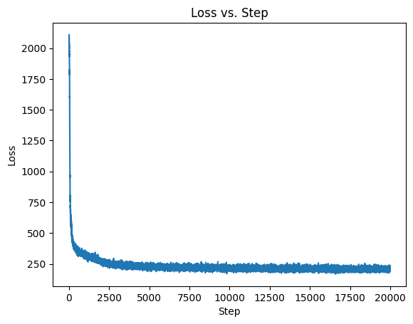
从图中可以看到，初始 loss 非常高，大约超过 2000，在前几百步内快速下降；到几千步后，loss 下降到约 200 多，后续在较低区间内缓慢下降并波动；到 20000 step 附近，loss 基本趋于稳定。这说明模型确实学到了 MNIST 条件概率路径上的向量场。

让我们来看看最终模型的输出结果！

# Play with these!
samples_per_class = 10
num_timesteps = 100
guidance_scales = [1.0, 3.0, 5.0]

visualize_output(
    model=dit,
    path=path,
    samples_per_class=samples_per_class,
    num_timesteps=num_timesteps,
    guidance_scales=guidance_scales,
)
plt.show()

模型输出结果如下图所示：

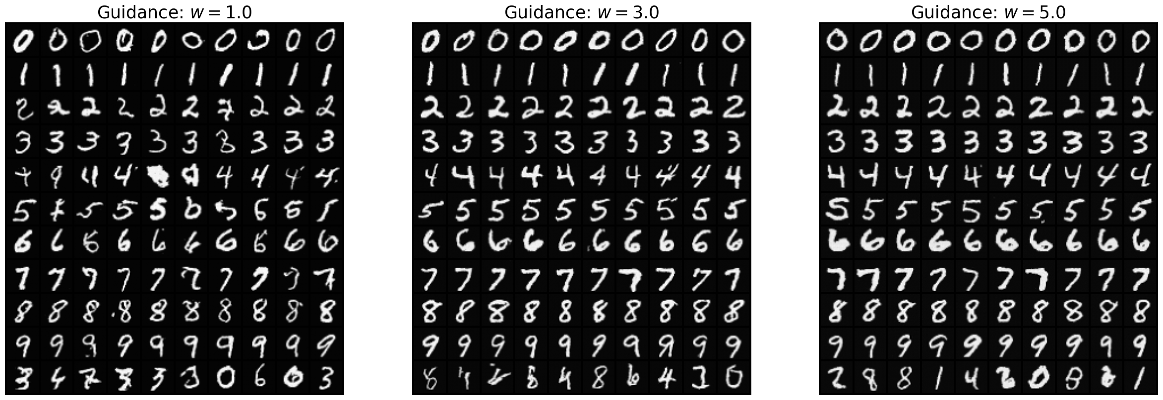
从图中我们可以看到：

一、当 $w=1.0$ 时

左侧面板 Guidance: w = 1.0 的特点是：

• 大部分样本已经能看出目标数字；
• 但有些数字还不够稳定；
• 个别样本存在形状扭曲、书写不规范甚至类别混淆的情况；
• 最后一行（null label）是无条件生成，因此类别比较杂乱。

这很符合理论预期。因为：

$${\tilde{u}}_t(x|y)=(1-w)u_t(x|\varnothing )+w{u}_t(x|y)$$

当 $w=1$ 时，有：

$${\tilde{u}}_t(x|y)=u_t(x|y)$$

也就是说，这里只是直接使用条件模型本身，没有额外强化类别条件。

所以此时生成结果通常：

• 多样性较高
• 类别一致性相对弱一些
• 图像质量可能还不错，但条件约束没那么强

二、当 $w=3.0$ 时

中间面板 Guidance: w = 3.0 明显比 $w=1.0$ 更稳定：

• 每一行数字基本都和目标类别一致；
• 字形更清晰；
• 不同样本之间虽然仍有变化，但整体更像 “标准手写数字”；
• 条件生成效果明显增强。

这通常是一个比较好的 guidance 区间，因为它在：

• 条件一致性
• 样本质量
• 样本多样性

之间取得了较好的平衡。

三、当 $w=5.0$ 时

右侧面板 Guidance: w = 5.0 可以看到：

• 类别一致性进一步增强；
• 数字看起来更 “坚定”、更 “像那个类”；
• 但有些类别开始出现更强的模式化；
• 多样性相比 $w=3.0$ 略有下降；
• 个别样本可能开始朝着 “过强约束” 方向发展。

这也是 CFG 的经典现象，随着 $w$ 增大，模型会更强烈地朝条件类别靠拢，但代价通常是：

• 多样性下降；
• 某些样本更容易变得僵硬；
• 再继续增大 $w$ 的话，可能还会出现失真、伪影、异常笔画等问题。

此外，每个面板的最后一行对应的其实是 y = 10 也就是 null label。这代表模型在 无条件模式 下的生成结果。因为没有指定 “你必须生成哪个数字”，所以这一行里会出现各种不同数字，比较杂乱，这是正常的。

它的存在有两个重要意义：

• 验证无条件分支确实学到了东西，如果 null label 完全生成不出数字，那说明 CFG 训练并不完整。
• 为 guided sampling 提供基线，CFG 公式本质上是利用 “无条件分支” 和 “有条件分支” 的差值来增强条件性。

从输出的结果来看，模型确实学会了条件生成，Class-Free Guidance 起作用了，整体训练质量已经比较不错了。

Part 4: Training a Variational Autoencoder

在这一节中，我们将为 MNIST 训练一个变分自编码器，也就是 VAE。在下一节中，我们会在 VAE 学到的 latent space 中训练一个 diffusion transformer。

回顾课程笔记，VAE 的整体结构包括两部分：

1. 一个 encoder：

$$q_{\varphi }(z|x)$$

它将输入图像 x 从形状 b 1 32 32 映射到两个输出：

• z_mean：b c h w
• z_logvar：一个可学习标量

注意，出于训练稳定性的考虑，同时也参考文献 [Robin+ 2022] 的做法，我们选择间接参数化 log-variance：

$$\log {\sigma }_{\varphi }(x)$$

2. 一个 decoder：

$$p_{\theta }(x|z)$$

它类似地将 latent z 映射到：

• x_mean：b 1 32 32
• x_logvar：一个可学习标量

和 diffusion transformer 的实现类似，我们会把 encoder 和 decoder 都构造成一系列 blocks。每个 block 包含若干个残差连接，随后是一个 attention layer，最后是一个 downsampling 或 upsampling layer。不过最后一个 block 例外，它不再继续下采样或上采样。

接下来，我们会逐个组件实现。每一部分都会先提供自然语言描述，然后让你补全具体实现。

Question 4.1: Residual Block

Your job：实现 ResidualBlock 类，使它完成如下流程：

0. 将输入保存为 x_skip，最后用于残差连接；

1. 应用某种归一化层。这里推荐使用 nn.GroupNorm(...)。当 num_groups = 1 时，它基本等价于对展平后的图像做 nn.LayerNorm；

2. 应用一个 kernel size 为 3 的卷积层；

3. 应用你喜欢的非线性激活函数；

4. 应用最后一个 $1\times 1$ 卷积，也就是 kernel size 为 1 的卷积；

5. 最后实现残差连接，返回前一步输出与 x_skip 的和。

class ResidualBlock(nn.Module):
  """ Two applications of LN + convolution + non-linearity + residual connection """
  def __init__(self, channels: int, act: nn.Module = nn.SiLU):
    super().__init__()

    # Init norm, convolutions, and activations
    self.norm = nn.GroupNorm(num_groups=1, num_channels=channels)
    self.conv1 = nn.Conv2d(
        in_channels=channels,
        out_channels=channels,
        kernel_size=3,
        padding=1
    )
    self.act = act()
    self.conv2 = nn.Conv2d(
        in_channels=channels,
        out_channels=channels,
        kernel_size=1
    )

    # Initialize the second convolution to zero - stabilizes training early on!
    nn.init.zeros_(self.conv2.weight)
    nn.init.zeros_(self.conv2.bias)

  def forward(self, x: torch.Tensor):
    # Res init
    x_skip = x

    # Norm
    x = self.norm(x)

    # First convolution
    x = self.conv1(x)

    # Activation
    x = self.act(x)

    # Second convolution
    x = self.conv2(x)

    # Return residual connection
    return x_skip + x

这个 ResidualBlock 是 VAE encoder 和 decoder 中最基础的构件。它的输入和输出形状保持一致，也就是说，它只改变特征表达，不改变空间分辨率，也不改变通道数。

Question 4.2: Attention Block

Your job：实现 AttnBlock 类，使其完成如下流程：

0. 将图像形状 b c h w 重排成 token 序列形状 b (h w) c，这里可以使用 einops.rearrange；

1. 保存 x_skip，用于下一步残差连接；

2. 应用归一化和 multi-head attention，也就是通过已有的 MHA 类实现；

3. 使用保存的 x_skip 做残差连接；

4. 再次保存 x_skip，用于下一步残差连接。

5. 应用归一化和 feedforward layer；

6. 使用保存的 x_skip 做残差连接。

class AttnBlock(nn.Module):
  def __init__(self, channels: int):
    super().__init__()

    # Reshape
    self.reshape1 = Rearrange('b c h w -> b (h w) c')

    # Norm + attention
    self.attn_norm = nn.LayerNorm(channels)
    self.attn = MHA(dim=channels, heads=4)

    # Norm + ff
    self.ff_norm = nn.LayerNorm(channels)
    self.ff = MLP([channels, 4 * channels, channels])


  def forward(self, x: torch.Tensor):
    b, c, h, w = x.shape
    x = self.reshape1(x)

    # Attention + residual connection
    x_skip = x
    x = self.attn_norm(x)
    x = self.attn(x)
    x = x_skip + x

    # Feedforward + residual connection
    x_skip = x
    x = self.ff_norm(x)
    x = self.ff(x)
    x = x_skip + x

    return rearrange(x, 'b (h w) c -> b c h w', h=h, w=w)

这个 AttnBlock 的输入和输出都是图像特征，但是 attention 本身更适合处理 token 序列，所以这个模块内部会先把二维图像特征展平成 token 序列，再做 self-attention，最后再恢复成图像形状。

Question 4.3: Encoder Block

Your job：实现 EncoderBlock 类，使它完成如下流程：

0. 应用两个 residual blocks；

1. 应用一个 attention block；

2. 如果 downsample_channels 不是 None，则应用一个下采样卷积。使用标准的 nn.Conv2d 即可，其中 kernel_size = 3，padding = 1，stride = 2。

class EncoderBlock(nn.Module):
  def __init__(self, in_channels: int, downsample_channels: Optional[int] = None):
    super().__init__()
    
    self.res1 = ResidualBlock(in_channels)
    self.res2 = ResidualBlock(in_channels)
    self.attn = AttnBlock(in_channels)

    if downsample_channels is not None:
      self.downsample = nn.Conv2d(
          in_channels=in_channels,
          out_channels=downsample_channels,
          kernel_size=3,
          stride=2,
          padding=1
      )
    else:
      self.downsample = nn.Identity()

  def forward(self, x: torch.Tensor):
    x = self.res1(x)
    x = self.res2(x)
    x = self.attn(x)
    x = self.downsample(x)
    return x

EncoderBlock 是 VAE encoder 的一个基础模块。它的作用是：先在当前分辨率下提取特征，再根据需要进行下采样。

Question 4.4: Encoder

Your job：实现 Encoder 类，使其完成如下流程：

0. 首先应用一个初始卷积层，将输入通道数，也就是 MNIST 中的 1 个通道，映射到初始 hidden channels；

1. 对每个 hidden channel 应用一个 encoder block，除了最后一个 block 之外，其余 block 都执行下采样；

2. 应用最后的 normalization 和 $1\times 1$ 输出卷积层，用来预测 z_mean；

3. 使用 self.logvar = nn.Parameter(torch.zeros(())) 定义一个可学习的标量 log-variance，并返回 z_mean 和 self.logvar。

class Encoder(nn.Module):
  def __init__(self, in_channels: int, hidden_channels: list[int]):
    super().__init__()

    # Initial conv2d
    self.init_conv = nn.Conv2d(in_channels = in_channels, out_channels = hidden_channels[0], kernel_size=3, padding=1, stride=1)

    # Initialize channels
    ch_in = hidden_channels
    ch_out = hidden_channels[1:] + [None]
    blocks = []
    for in_c, out_c in zip(ch_in, ch_out):
      blocks.append(EncoderBlock(in_c, out_c))
    self.blocks = nn.ModuleList(blocks)

    # Predict z_mean
    z_dim = hidden_channels[-1]
    self.z_mean = nn.Sequential(
      nn.GroupNorm(1, z_dim),
      nn.Conv2d(in_channels = z_dim, out_channels = z_dim, kernel_size=1, stride=1, padding=0),
    )

    # Scalar log-variance
    self.logvar = nn.Parameter(torch.zeros(()))

  def forward(self, x: torch.Tensor):
    x = self.init_conv(x)

    for block in self.blocks:
      x = block(x)

    z_mean = self.z_mean(x)
    return z_mean, self.logvar

Encoder 的作用是把输入图像 $x$ 编码成 latent distribution 的参数。对于 VAE 来说，encoder 不是直接输出一个确定性 latent，而是输出近似后验分布：

$$q_{\varphi }(z|x)$$

在当前实现中，它返回：

• z_mean：latent 的均值
• logvar：latent 的 log-variance

也就是可以理解为：

$$q_{\varphi }(z|x)=\mathcal{N}(z_{\text{mean}},{\sigma }^{2}I)$$

其中 $\log {\sigma }^2$ 由 self.logvar 表示。

Question 4.5: Decoder Block

Your job：实现 DecoderBlock 类，使其完成如下流程：

0. 应用两个 residual blocks；

1. 应用一个 attention block；

2. 如果 upsample_channels 不是 None，则应用一个上采样模块，例如先使用 nn.Upsample，再接一个标准卷积层。

class DecoderBlock(nn.Module):
  def __init__(self, in_channels: int, upsample_channels: Optional[int] = None):
    super().__init__()
    self.res1 = ResidualBlock(in_channels)
    self.res2 = ResidualBlock(in_channels)
    self.attn = AttnBlock(in_channels)
    if upsample_channels is not None:
      self.upsample = nn.Sequential(
        nn.Upsample(scale_factor=2, mode='nearest'),
        nn.Conv2d(in_channels=in_channels, out_channels=upsample_channels, kernel_size=3, padding=1, stride=1),
      )
    else:
      self.upsample = None

  def forward(self, x: torch.Tensor):
    x = self.res1(x)
    x = self.res2(x)
    x = self.attn(x)

    if self.upsample is not None:
      x = self.upsample(x)

    return x

DecoderBlock 是 VAE decoder 中的基本模块。它的结构和 EncoderBlock 非常相似，区别在于，EncoderBlock 最后可选执行的是 downsample，而 DecoderBlock 最后可选执行的是 upsample。

Your job：实现 Decoder 类，使其完成如下流程：

0. 对每个 hidden channel 应用一个 decoder block，除了最后一个 block 之外，其余 block 都执行上采样；

1. 应用最后的 normalization 和 $1\times 1$ 输出卷积层，用来预测 x_mean；

3. 使用 self.logvar = nn.Parameter(torch.zeros(())) 定义一个可学习的标量 log-variance，并返回 x_mean 和 self.logvar。

class Decoder(nn.Module):
  def __init__(self, out_channels: int, hidden_channels: list[int]):
    super().__init__()

    # Initialize channels
    ch_in = hidden_channels
    ch_out = hidden_channels[1:] + [None]
    blocks = []
    for in_c, out_c in zip(ch_in, ch_out):
      blocks.append(DecoderBlock(in_c, out_c))
    self.blocks = nn.ModuleList(blocks)

    # Predict mean
    x_dim = hidden_channels[-1]
    self.x_mean = nn.Sequential(
      nn.GroupNorm(1, x_dim),
      nn.Conv2d(in_channels = x_dim, out_channels = out_channels, kernel_size=1, stride=1, padding=0),
    )

    # Scalar log-variance
    self.logvar = nn.Parameter(torch.zeros(()))

  def forward(self, x: torch.Tensor):
    for block in self.blocks:
      x = block(x)

    x_mean = self.x_mean(x)
    return x_mean, self.logvar

Decoder 是 VAE 的解码器部分，对应概率模型：

$$p_{\theta }(x|z)$$

它的作用是将 latent variable z 解码回图像空间，并输出重建图像分布的参数。

在当前实现中，它返回：

• x_mean：b 1 32 32
• logvar：标量

也就是说，它建模的是：

$$p_{\theta }(x|z)=\mathcal{N}(x_{\text{mean}},{\sigma }_x^{2}I)$$

其中 $x_{\text{mean}}=g_{\theta }(z)$ ，而 ${\sigma }_x^2$ 由一个可学习标量 self.logvar 控制。

Question 4.7: Putting It Together

最后，我们将上面实现的子组件组合起来，完成 VAE 类。

Your job：现 VAE.compute_loss(...)，也就是实现正文中 display (85) 给出的 VAE 损失：

$$L_{\text{VAE}}(\varphi ,\theta )$$

class VAE(nn.Module):
  def __init__(self, data_channels: int, hidden_channels: list[int], beta: float = 0.1):
    super().__init__()
    self.beta = beta

    # Encoder
    self._encoder = Encoder(data_channels, hidden_channels)

    # Decoder
    self._decoder = Decoder(data_channels, list(reversed(hidden_channels)))

  def encode(self, x: torch.Tensor):
    return self._encoder(x)

  def decode(self, z: torch.Tensor):
    return self._decoder(z)

  def forward(self, x: torch.Tensor):
    z_mean, z_logvar = self.encode(x)
    z = z_mean + torch.exp(0.5 * z_logvar) * torch.randn_like(z_mean)
    x_mean, x_logvar = self.decode(z)
    return z_mean, z_logvar, x_mean, x_logvar

  def compute_loss(self, z_mean: torch.Tensor, z_logvar: torch.Tensor, x_mean: torch.Tensor, x_logvar: torch.Tensor, x_true: torch.Tensor):
    """ See display 85 from the text """
    # KL loss
    kl_loss = 0.5 * torch.sum(
        torch.exp(z_logvar) + z_mean ** 2 - 1.0 - z_logvar,
        dim=tuple(range(1, z_mean.ndim))
    )
    kl_loss = self.beta * kl_loss.mean()

    # Reconstruction loss
    recon_loss = 0.5 * torch.sum(
        torch.exp(-x_logvar) * (x_true - x_mean) ** 2 + x_logvar,
        dim=tuple(range(1, x_true.ndim))
    )
    recon_loss = recon_loss.mean()

    return kl_loss + recon_loss

这个 VAE 类由两部分组成：

• Encoder：$q_{\varphi }(z|x)$
• Decoder：$p_{\theta }(x|z)$

encoder 将输入图像编码成 latent distribution，decoder 从 latent sample 中重建图像。

VAE 的损失通常由两部分组成：

$$L_{\text{VAE}}=\beta D_{\text{KL}}(q_{\varphi }(z|x)\Vert p(z))-{\mathbb{E}}_{q_{\varphi }(z|x)}[\log p_{\theta }(x|z)]$$

在代码中对应：

return kl_loss + recon_loss

1. KL Loss

kl_loss = 0.5 * torch.sum(
    torch.exp(z_logvar) + z_mean ** 2 - 1.0 - z_logvar,
    dim=tuple(range(1, z_mean.ndim))
)
kl_loss = self.beta * kl_loss.mean()

这一项衡量 encoder 得到的 posterior：

$$q_{\varphi }(z|x)=\mathcal{N}(z_{\text{mean}},\exp (z_{\text{logvar}})I)$$

和标准正态先验：

$$p(z)=\mathcal{N}(0,I)$$

之间的距离。

两个对角高斯之间的 KL 散度为：

$$D_{\text{KL}}(q_{\varphi }(z|x)\Vert p(z))=\frac{1}{2}\sum _i\left(\exp (z_{\text{logvar},i})+z_{\text{mean},i}^2-1-z_{\text{logvar},i}\right)$$

虽然这里 z_logvar 是一个标量，但 PyTorch 会自动广播到 z_mean 的形状，因此可以直接写：

torch.exp(z_logvar) + z_mean ** 2 - 1.0 - z_logvar

然后对除 batch 维之外的所有维度求和：

dim=tuple(range(1, z_mean.ndim))

最后再对 batch 求平均。

这里乘上 self.beta 表示这是一个 beta-VAE 风格的损失：

$$\beta D_{\text{KL}}(q_{\varphi }(z|x)\Vert p(z))$$

默认 beta = 0.1 说明这里对 KL 的约束相对弱一些，更鼓励模型先学好重建质量。

2. Reconstruction Loss

recon_loss = 0.5 * torch.sum(
    torch.exp(-x_logvar) * (x_true - x_mean) ** 2 + x_logvar,
    dim=tuple(range(1, x_true.ndim))
)
recon_loss = recon_loss.mean()

这一项来自高斯重建分布的负对数似然：

$$-\log p_{\theta }(x|z)$$

由于：

$$p_{\theta }(x|z)=\mathcal{N}(x_{\text{mean}},\exp (x_{\text{logvar}})I)$$

所以负对数似然为：

$$-\log p_{\theta }(x|z)=\frac{1}{2}\sum _i\left[\exp (-x_{\text{logvar}})(x_i-x_{\text{mean},i}{)}^2+x_{\text{logvar}}\right]$$

这里省略了常数项：

$$\frac{1}{2}\log (2\pi )$$

因为它不影响模型优化。

这一项的作用是让 decoder 输出的 x_mean 尽可能接近真实图像 x_true。

同时，因为 x_logvar 是可学习参数，loss 中必须包含 x_logvar 项。否则模型可能通过无限增大方差来降低误差项，导致训练退化。

在训练之前，我们创建一个新的 Trainer 子类，用来训练 VAE。同时，我们还会创建一个辅助函数，用于可视化在学到的 latent space 中进行插值的效果。

class MNISTVAETrainer(Trainer):
  def __init__(self, mnist_sampleable: LabeledSampleable, batch_size: int = 64, **kwargs):
    super().__init__(**kwargs)
    self.mnist = mnist_sampleable
    self.batch_size = batch_size

  def get_train_loss(self):
    """ See display 85 from the text """
    x, y = self.mnist.sample(self.batch_size)
    z_mean, z_std, x_mean, x_std = self.model(x)
    return self.model.compute_loss(z_mean, z_std, x_mean, x_std, x)

  @torch.no_grad()
  def checkpoint(self, step: int):
    # Save model
    torch.save(self.model.state_dict(), os.path.join(self.output_dir, f'step_{step:06d}_model.pt'))
    torch.save(self.opt.state_dict(), os.path.join(self.output_dir, f'step_{step:06d}_opt.pt'))

    # Save output visualization, using x_mean as reconstruction
    b = 10
    x, _ = self.mnist.sample(b)
    _, _, x_mean, _ = self.model(x)
    x_all = torch.cat([x, x_mean], dim=0)
    grid = make_grid(x_all, nrow=b, normalize=True, value_range=(0,1))
    plt.imshow(grid.permute(1, 2, 0).cpu(), cmap="gray")
    plt.axis("off")
    plt.title("VAE Reconstruction")
    plt.savefig(os.path.join(self.output_dir, f'step_{step:06d}_output.png'))
    plt.close()

@torch.no_grad()
def visualize_latent_interpolation(x1: torch.Tensor, x2: torch.Tensor, vae: VAE, n_steps: int, save_path: Optional[str] = None):
   z1_mean, z1_logvar = vae.encode(x1)
   z1 = z1_mean + torch.exp(0.5 * z1_logvar) * torch.randn_like(z1_mean) # 1 c h w

   z2_mean, z2_logvar = vae.encode(x2)
   z2 = z2_mean + torch.exp(0.5 * z2_logvar) * torch.randn_like(z2_mean) # 1 c h w

   lambdas = torch.linspace(0, 1, n_steps).to(z1.device)
   zs = (1 - lambdas) * z1.unsqueeze(-1) + lambdas * z2.unsqueeze(-1) # 1 c h w n_steps
   zs = rearrange(zs, '1 c h w n -> n c h w')
   samples, _ = vae.decode(zs) # n_steps 1 h w

   grid = make_grid(samples, nrow=n_steps, normalize=True, value_range=(0, 1))
   plt.figure(figsize=(n_steps * 2, 2))
   plt.imshow(grid.permute(1, 2, 0).cpu(), cmap="gray")
   plt.axis("off")
   plt.title("Latent Interpolation")
   if save_path is not None:
       plt.savefig(save_path)
       plt.close()
   else:
       plt.show()
   return samples

最后，让我们开始训练 VAE。

# Create dataset + VAE
device = torch.device('cuda')
mnist = MNISTSampler().to(device)
vae = VAE(
   data_channels = 1,
   hidden_channels = [16, 32, 64, 128],
   beta = 10.0,
).to(device)

# Create Trainer + train
trainer = MNISTVAETrainer(
    mnist_sampleable = mnist,
    batch_size = 64,
)
losses, steps = trainer.train(
   model = vae,
   num_steps = 5000,
   lr = 1e-3,
   warmup_steps = 500,
   ckpt_every = 250,
)
plt.plot(steps, losses)
plt.xlabel("Step")
plt.ylabel("Loss")
plt.show()

训练损失曲线如下图所示：

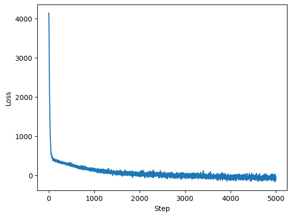
这条曲线整体来看是正常的，具备一个健康训练曲线的典型特征：快速下降 → 持续优化 → 后期趋于稳定 → 小幅随机波动，没有出现 loss 爆炸、NaN 等现象，所以我们当前 VAE 的训练过程是有效的。

训练过程中 checkpoint 保存的 reconstruction 图像如下：

可以看到重建图像足够清晰，这说明模型确实学到了有用的 latent space。

我们来尝试在 VAE 学到的 latent space 中做插值，观察下 decoder 解码后的图像变化是否平滑自然：

# Perform interpolation in the latent space
vae.eval()
samples, _ = mnist.sample(2)
interpolated_samples = visualize_latent_interpolation(
   x1 = samples[:1],
   x2 = samples[1:2],
   vae = vae,
   n_steps = 10,
) # n_steps 1 h w

可视化图如下所示：

从图中可以看出：

• 左边起始图像明显更像数字 1
• 右边终止图像明显更像数字 2
• 中间的若干图像并不是突然跳变，而是逐渐地从 “1” 的形态过渡到 “2” 的形态

这说明：

1. latent space 具有连续性

如果 latent space 是杂乱无章的，那么在两个 latent 之间做线性插值时，解码出来的图像通常会变得非常混乱，甚至完全不像数字。

但这里的结果表明，随着插值逐步推进，图像形状也逐步变化，这说明 VAE 学到的 latent manifold 是比较平滑的。

2. latent space 具有一定语义结构

这里不是简单地做像素空间插值，而是在 latent space 中插值。
如果在原始像素空间直接插值，通常会得到 “两个数字重影叠加” 的模糊结果；而在 latent space 中插值，模型学到的是更高层的结构信息，所以过渡更接近 “数字类别与书写形态的渐变”。

从这张图可以观察到：

• 前几步仍然保留了 “1” 的细长竖线特征
• 中间几步开始出现弯折、顶部弧形或笔画转向
• 后几步逐渐形成 “2” 的整体轮廓

这种现象说明 VAE 学到的不只是像素重建，而是某种低维语义表示。

这张图实际上是对 VAE 训练效果的一个非常重要的验证。它说明了：

1. encoder 学会了把不同数字映射到一个有结构的 latent space；

2. decoder 学会了从 latent 表示中恢复出合理的 MNIST 图像；

3. latent space 中的局部区域具有一定平滑性和语义一致性；

4. 因而这个 latent space 是适合后续进行生成建模的。

这也是为什么下一部分我们会进一步在 latent space 中训练 diffusion transformer。因为相比直接在像素空间建模，latent space 维度更低、结构更规整、更容易学习高层语义变化。

Part 5: Training a Latent Diffusion Model

在这一节中，我们将在训练好的 VAE 的 latent space 内部训练一个 diffusion transformer。幸运的是，大部分工作我们前面已经完成了！现在剩下的事情就是把所有组件组合起来：VAE + latent probability path + diffusion transformer。

Question 5.1: Latent Diffusion Trainer

下面是 LatentCFGTrainer 的部分实现。它是 CFGTrainer 的扩展版本，用于在 VAE 的 latent space 中训练模型。

Your job：实现 LatentCFGTrainer.get_train_loss。

Hint：

1. 参考 CFGTrainer.get_train_loss 的实现，但是这里不再调用 self.path.p_data.sample(...)，而是需要直接从 MNIST 中采样图像，然后通过 VAE encoder 得到 latent 表示。

2. 注意：调用 vae.encode 时，一定要放在 torch.no_grad() 下。

class LatentCFGTrainer(Trainer):
    def __init__(
        self,
        mnist: MNISTSampler,
        vae: VAE,
        path: GaussianConditionalProbabilityPath,
        eta: float,
        null_label: int,
        eps: float = 0.001,
        **kwargs
    ):
        assert eta > 0 and eta < 1
        super().__init__(**kwargs)
        self.mnist = mnist
        self.vae = vae
        self.path = path
        self.eta = eta
        self.eps = eps
        self.path = path
        self.null_label = null_label

    @torch.no_grad()
    def visualize_samples(self, save_path: str, samples_per_class: int = 10, num_timesteps: int = 100, guidance_scales: List[float] = [1.0, 3.0, 5.0], use_tqdm = False):
      # Graph
      fig, axes = plt.subplots(1, len(guidance_scales), figsize=(10 * len(guidance_scales), 10))

      for idx, w in enumerate(guidance_scales):
          # Setup ode and simulator
          ode = CFGVectorFieldODE(self.model, guidance_scale=w, null_label=10)
          simulator = EulerSimulator(ode)

          # Sample initial conditions
          y = torch.tensor([0, 1, 2, 3, 4, 5, 6, 7, 8, 9, 10], dtype=torch.int64).repeat_interleave(samples_per_class).to(device)
          num_samples = y.shape[0]
          z0 = self.path.p_simple.sample(num_samples)

          # Simulate
          ts = torch.linspace(0,0.999,num_timesteps).view(1, -1, 1, 1, 1).expand(num_samples, -1, 1, 1, 1).to(device)
          z1 = simulator.simulate(z0, ts, y=y, use_tqdm=use_tqdm)

          # Decode
          x1, _ = self.vae.decode(z1)

          # Plot
          v_min, v_max = x1.min(), x1.max()
          x1 = (x1 - v_min) / (v_max - v_min)
          grid = make_grid(x1, nrow=samples_per_class, normalize=True, value_range=(0,1))
          axes[idx].imshow(grid.permute(1, 2, 0).cpu(), cmap="gray")
          axes[idx].axis("off")
          axes[idx].set_title(f"Guidance: $w={w:.1f}$", fontsize=25)

      # Save
      if save_path is not None:
          plt.savefig(save_path)
          plt.close()
      else:
        plt.show()

    plt.show()

    def checkpoint(self, step: int):
      # Save model
      torch.save(self.model.state_dict(), os.path.join(self.output_dir, f'step_{step:6d}_model.pt'))
      torch.save(self.opt.state_dict(), os.path.join(self.output_dir, f'step_{step:6d}_opt.pt'))

      # Save output visualization
      self.visualize_samples(save_path=os.path.join(self.output_dir, f'step_{step:6d}_output.png'))

    def get_train_loss(self, batch_size: int) -> torch.Tensor:
        # Get device from model
        device = next(self.model.parameters()).device

        # Step 1: Sample z, y from MNIST + encode
        with torch.no_grad():
          x, y = self.mnist.sample(batch_size)
          x = x.to(device)
          y = y.to(device)

          z_mean, z_logvar = self.vae.encode(x)
          z = z_mean + torch.exp(0.5 * z_logvar) * torch.randn_like(z_mean)

        # Step 2: Set each label to 10 (i.e., null) with probability eta
        mask = torch.rand(batch_size, device=device) < self.eta
        y = y.clone()
        y[mask] = self.null_label

        # Step 3: Sample t and x
        t = self.eps + (1.0 - 2.0 * self.eps) * torch.rand(batch_size, device=device)
        x = self.path.sample_conditional_path(z, t)

        # Step 4: Regress and output loss
        pred_vector_field = self.model(x, t, y)
        target_vector_field = self.path.conditional_vector_field(x, z, t)

        loss = torch.mean(
            torch.sum(
                (pred_vector_field - target_vector_field) ** 2,
                dim=tuple(range(1, pred_vector_field.ndim))
            )
        )

        return loss

这一题的核心思想是：把 pixel-space CFG training 改成 latent-space CFG training。

前面在像素空间中训练时，我们的训练目标是：

$$u_t^{\theta }(x_t|y)\approx u_t^{\text{ref}}(x_t|x_1)$$

其中 $x_1$ 是真实 MNIST 图像。

现在进入 latent diffusion 后，真实数据不再是像素图像 $x$ ，而是 VAE encoder 得到的 latent 表示 $z$ 。因此训练目标变成：

$$u_t^{\theta }(z_t|y)\approx u_t^{\text{ref}}(z_t|z_1)$$

其中 $z_1\sim q_{\varphi }(z|x)$ 。

1. 从 MNIST 采样并编码到 latent space

with torch.no_grad():
  x, y = self.mnist.sample(batch_size)
  x = x.to(device)
  y = y.to(device)

  z_mean, z_logvar = self.vae.encode(x)
  z = z_mean + torch.exp(0.5 * z_logvar) * torch.randn_like(z_mean)

这里首先从 MNIST 中采样真实图像 x 和标签 y，然后通过训练好的 VAE encoder 得到 z_mean 和 z_logvar，再使用 reparameterization trick 采样 latent：

$$z=z_{\text{mean}}+\exp (0.5z_{\text{logvar}})ϵ,ϵ\sim \mathcal{N}(0,I)$$

2. Label dropout

mask = torch.rand(batch_size, device=device) < self.eta
y = y.clone()
y[mask] = self.null_label

这一步和前面的 CFG 训练完全一致。

对于 MNIST，真实标签是 0~9，而 null label 是 10，训练时以概率 $\eta$ 将真实标签替换成 null label。这样模型可以同时学习条件向量场 $u_t(z|y)$ 和无条件向量场 $u_t(z|\varnothing )$ ，后续推理时就可以使用 CFG 公式：

$${\tilde{u}}_t(z|y)=(1-w)u_t(z|\varnothing )+w{u}_t(z|y)$$

3. 构造 latent conditional path

t = self.eps + (1.0 - 2.0 * self.eps) * torch.rand(batch_size, device=device)
x = self.path.sample_conditional_path(z, t)

这里变量名仍然写成 x，但它已经不是 pixel image，而是 latent path 上的中间状态。更准确地说，它应该叫 zt，也就是：

$$z_t={\alpha }_{t}z+{\beta }_tϵ$$

在当前线性高斯路径下：

$${\alpha }_t=t,{\beta }_t=1-t$$

所以：

$$z_t=tz+(1-t)ϵ.$$

4. 回归参考向量场

pred_vector_field = self.model(x, t, y)
target_vector_field = self.path.conditional_vector_field(x, z, t)

这里模型输入的是 latent 中间状态 x、时间 t 和标签 y，输出也是 latent space 中的向量场 pred_vector_field。

参考向量场来自概率路径：

$$u_t^{\text{ref}}(z_t|z)$$

也就是：

self.path.conditional_vector_field(x, z, t)

最终模型通过 MSE 学习这个向量场。

5. Loss 计算

loss = torch.mean(
    torch.sum(
        (pred_vector_field - target_vector_field) ** 2,
        dim=tuple(range(1, pred_vector_field.ndim))
    )
)

这里和前面的 CFGTrainer 一致，先对除 batch 维之外的所有 latent 维度求平方误差和，再对 batch 求平均。

一切准备就绪！让我们开始训练。

# Finally, let's train!

vae = vae.to(device) # VAE(data_channels = 1, hidden_channels = [16, 32, 64, 128], beta = 1.0)

# Initialize latent probability path
c = 128
img_size = 4

path = GaussianConditionalProbabilityPath(
    p_data = None,
    p_simple_shape = [c, img_size, img_size],
    alpha = LinearAlpha(),
    beta = LinearBeta()
).to(device)

# Initialize model
dit = DiffusionTransformerFlowModel(
    img_size = img_size,
    patch_size = 1,
    num_layers = 8,
    c = c,
    dim = 256,
    heads = 8,
    final_dim = 10,
    n_classes = 11,
).to(device)

# Dataset
mnist = MNISTSampler().to(device)

# Initialize trainer
trainer = LatentCFGTrainer(
    mnist = mnist,
    vae = vae,
    path = path,
    eta=0.35,
    null_label=10
)

# Train! You should have reasonable results in ~15 A100 minutes
losses, steps = trainer.train(model=dit, num_steps = 10000, lr=0.4e-3, batch_size=256, ckpt_every=500)

plt.plot(steps, losses)
plt.xlabel("Step")
plt.ylabel("Loss")
plt.title("Loss vs. Step")
plt.show()

训练损失曲线如下图所示：

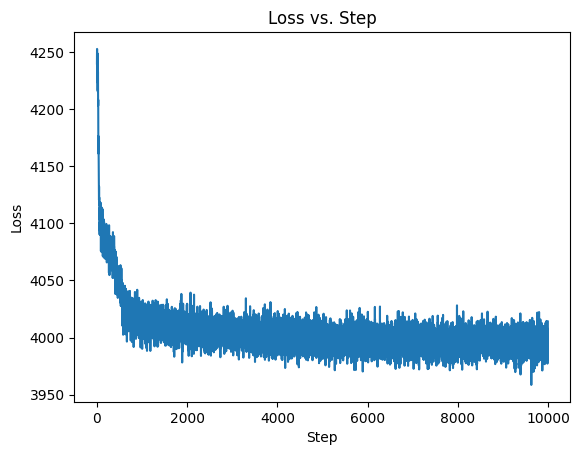
从上面的曲线我们可以看到 loss 从大约 4250 快速下降到 4000 附近，然后在 4000 左右震荡，这个现象整体是合理的。

Note：训练时间相比之前也是有减少的，博主之前在像素空间训练大约 ~1h，现在在 VAE latent space 下仅 ~35min。

训练过程中不同 guidance scale 的生成结果如下所示：

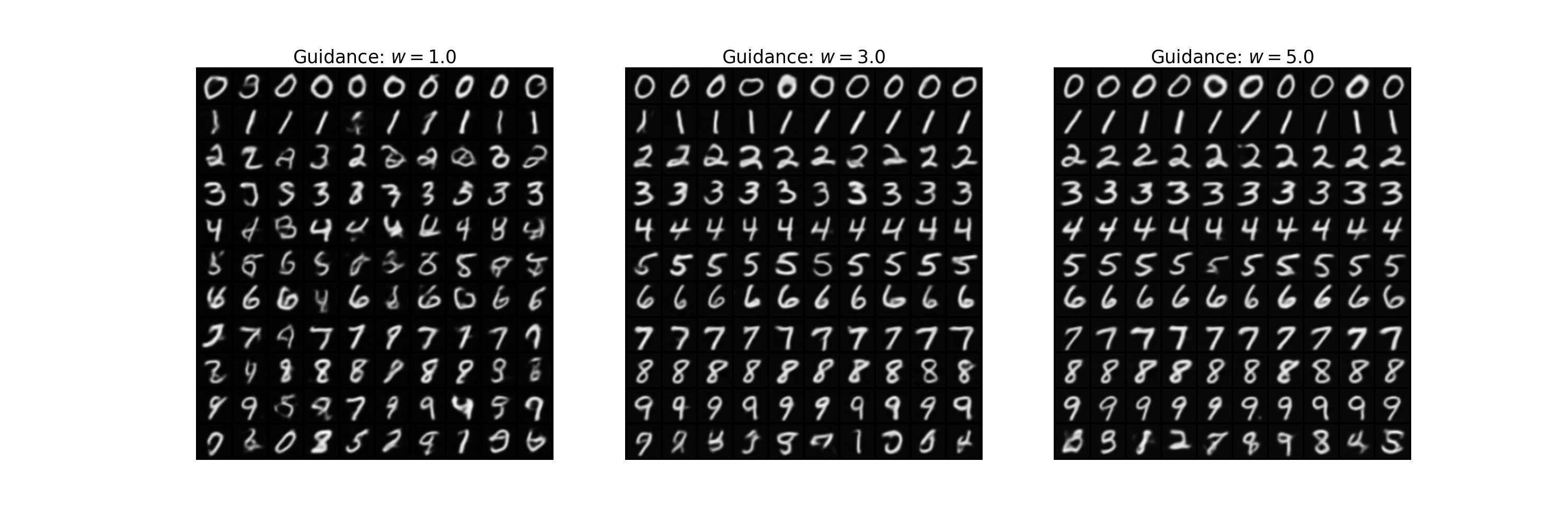
前面我们直接在像素空间训练过 DiT，现在这里是在 VAE latent space 里训练 DiT。

第一，类别控制依然有效。说明 VAE latent space 保留了足够的数字语义信息，DiT 可以在其中学习条件生成。

第二，生成图像整体更平滑。这部分平滑性主要来自 VAE decoder，因为 decoder 输出的是重建分布的均值，天然会带一点 VAE 风格的柔和感。

第三，latent space 中的生成更加 “结构化”。前面 latent interpolation 已经证明 VAE latent space 是连续的，因此 diffusion model 在这个空间中采样时，更容易沿着合理的数字 manifold 运动。

第四，最终图像质量受两个模型共同影响：Latent DiT 决定生成什么 latent，VAE decoder 决定 latent 如何还原成图像，所以如果后续想进一步提升生成质量，除了训练 latent DiT，也可以提升 VAE decoder 的重建质量。

OK，以上就是本次作业 Lab 3: Diffusion Transformer and VAEs 的全部实现了。

结语

本次 Lab 3 从 Conditional Diffusion Transformer 与 VAE Latent Modeling 出发，完整构建了一个现代生成模型的工程化流程。我们从最基础的条件生成问题出发，将无条件建模扩展为 $p(x\mid y)$ ，引入类别信息作为控制信号，使模型具备可控生成能力。这一变化本质上是从 “建模数据分布” 走向 “建模可控数据分布”，也是现代生成式 AI 的核心方向之一。

在训练机制上，我们引入了 Classifier-Free Guidance（CFG），通过在训练阶段随机丢弃条件，并在推理阶段对条件差异进行放大，实现了无需额外模型即可增强生成质量与可控性的效果。从数学角度来看，CFG 本质是在向量场空间中对 “条件方向” 进行线性增强，使模型在保持无条件生成能力的同时，实现更强的条件对齐能力。

在模型结构方面，本实验实现了完整的 Diffusion Transformer（DiT）框架，将图像从 pixel space 切分为 patch token，并通过 Transformer 进行建模，同时融合时间嵌入与类别嵌入来调制生成过程。整个网络最终学习的是一个条件向量场 $u_{\theta }(x_t,t,y)$ ，用于描述从噪声到数据分布的演化方向。这种设计使得扩散 / flow 模型可以自然地与 Transformer 架构结合，从而具备更强的表达能力与扩展性。

在此基础上，引入 VAE latent space 是本次实验的另一个关键改进。通过将图像压缩到低维 latent 表示，模型不再直接在高维像素空间中学习，而是在结构更平滑、更语义化的 latent manifold 上进行建模。这一转换显著降低了计算复杂度，同时提升了生成过程的稳定性，使 diffusion trajectory 更符合数据的内在结构。整体生成流程也因此变为 “image → latent → DiT → latent → decoder → image”的标准现代生成范式。

从实验结果来看，CFG scale 的调节直接影响生成质量与多样性之间的权衡，而 latent space 中的生成效果明显优于像素空间训练，这进一步验证了表示学习在生成模型中的关键作用。同时，VAE decoder 对输出图像的平滑化影响也表明，最终生成质量是由表示学习与生成模型共同决定的，而不仅仅依赖扩散网络本身。

总体而言，本次 Lab 不仅完成了一个 Diffusion Transformer 的完整实现，更重要的是串联了现代生成模型的三大核心组件：latent representation learning、Transformer-based vector field modeling，以及 classifier-free guidance conditioning。这些模块共同构成了当前主流图像生成系统（如 Stable Diffusion 系列）的基础结构，也为后续更大规模生成模型的理解与实现打下了完整基础🤗。

参考

• https://github.com/eje24/iap-diffusion-labs