前言

本篇文章记录 MIT S.184 作业 Lab 3: Diffusion Transformer and VAEs 的实现，和大家一起分享交流😄。

reference：https://github.com/eje24/iap-diffusion-labs

Lab 3: A Conditional Generative Model for Images

欢迎来到 Lab 3！在上一个实验中，我们研究了 toy 二维数据分布上的 无条件生成。在本实验中，我们将研究 MNIST 手写数字图像上的 条件生成。

每一张 MNIST 图像不再是二维数据，而是 $32\times 32=1024$ 维的数据！新的、更具挑战性的设定要求我们格外注意以下两点：

1. 为了处理 条件生成，我们将使用 classifier-free guidance，简称 CFG，详见 Part 2.1。
2. 为了参数化高维图像数据上的可学习向量场，简单的 MLP 已经不够用了。因此，我们将采用 diffusion transformer 架构，详见 Part 3。

老规矩，我们先为 Lab Three 准备一些必要的环境依赖：

import os
from abc import ABC, abstractmethod
from typing import Optional, List, Type, Tuple, Dict
import math
import uuid
import random

import numpy as np
from matplotlib import pyplot as plt
from matplotlib.axes._axes import Axes
import torch
import torch.nn as nn
import torch.distributions as D
from torch.func import vmap, jacrev
from tqdm import tqdm
import seaborn as sns
from sklearn.datasets import make_moons, make_circles
from torchvision import datasets, transforms
from torchvision.utils import make_grid
from einops import rearrange
from einops.layers.torch import Rearrange

Part 0: Recycling Components from Previous Labs

在这一节中，我们将重新导入 Lab One 和 Lab Two 中使用过的组件。在这个过程中，我们会做一些重要更新。

首先，让我们回顾一下 Lab One 和 Lab Two 中的 Sampleable 类。下面，我们将它称为 OldSampleable。

class Sampleable(ABC):
    """
    Distribution which can be sampled from
    """
    @abstractmethod
    def sample(self, num_samples: int) -> torch.Tensor:
        """
        Args:
            - num_samples: the desired number of samples
        Returns:
            - samples: b d
        """
        pass

这段代码重新定义了一个 Sampleable 抽象基类，表示 “可以从中采样的分布”。在前两个 lab 中，我们经常把一个分布抽象成 Sampleable，只要某个类实现了：

sample(self, num_samples: int)

就可以被统一当作一个可采样分布使用。

例如前面 Lab Two 中的

Gaussian
GaussianMixture
MoonsSampleable
CirclesSampleable
CheckerboardSampleable

本质上都属于 Sampleable，因为它们都能返回一批样本。

正如我们很快会看到的，像 MNIST 这样的数据集不仅包含图像，也就是这里的手写数字图像，还包含类别标签，也就是一个从 0 到 9 的数值，用来表示这张图像对应哪个数字。

因此，我们将把 Sampleable 泛化为 LabeledSampleable，使它也能够容纳这些标签。旧的 Sampleable.sample 方法只返回 samples: torch.Tensor，而新的 LabeledSampleable.sample 会同时返回 samples: torch.Tensor 以及 labels: Optional[torch.Tensor]。这样一来，我们就可以形式化地把每一个这样的 Sampleable 实例理解为：从一个关于数据和标签的 联合分布 中采样。

下面我们实现新的 LabeledSampleable。

class LabeledSampleable(ABC):
    """
    Distribution which can be sampled from
    """
    @abstractmethod
    def sample(self, num_samples: int) -> Tuple[torch.Tensor, Optional[torch.Tensor]]:
        """
        Args:
            - num_samples: the desired number of samples
        Returns:
            - samples: b d
            - labels: b
        """
        pass

这段代码定义了一个新的抽象接口 LabeledSampleable，用于表示 “可以同时采样数据和标签的分布”。在前两个 Lab 中，我们主要处理无条件生成任务，因此只需要从分布中采样数据点：

samples = p.sample(num_samples)

但在 Lab Three 中，我们要做的是 MNIST 图像的 条件生成。也就是说，我们希望模型不仅能生成一张手写数字图片，还能根据指定类别生成对应数字，例如：

给定 label = 3，生成数字 3 的图像
给定 label = 7，生成数字 7 的图像

因此，采样接口需要同时返回图像和标签。

对于某些分布，例如高斯分布，其实并不适合去考虑标签。正因如此，我们会选择把 Gaussian 类实现成一个简单的 Sampleable。

再次强调一下，把一个简单高斯分布 “对象化” 其实有些形式化，这主要是出于教学目的，同时也是为了强调：在我们的理解框架中，分布本身应该被当作一等对象来对待。

在实际工程中，更常见也更实用的做法，是直接使用库函数，例如 torch.randn 或 torch.randn_like。

class IsotropicGaussian(nn.Module, Sampleable):
    """
    Sampleable wrapper around torch.randn
    """
    def __init__(self, shape: List[int], std: float = 1.0):
        """
        shape: shape of sampled data
        """
        super().__init__()
        self.shape = shape
        self.std = std
        self.dummy = nn.Buffer(torch.zeros(1)) # Will automatically be moved when self.to(...) is called...

    def sample(self, num_samples) -> torch.Tensor:
        return self.std * torch.randn(num_samples, *self.shape).to(self.dummy.device)

这段代码定义了一个各向同性高斯分布类 IsotropicGaussian，它本质上是对 torch.randn 的简单封装。

它继承了两个类：

class IsotropicGaussian(nn.Module, Sampleable):

其中 nn.Module 说明它是一个 PyTorch 模块，可以使用 .to(device) 移动到 GPU 或 CPU；Sampleable 说明它实现了统一的采样接口：

sample(num_samples)

我们也会像前面几个 lab 一样，实现一个 高斯混合模型，也就是 GMM。对于 GMM 来说，标签可以很自然地由对应的混合分量产生：样本来自第几个高斯分量，它的标签就是几。

GMM 可以帮助我们在正式进入图像任务之前，先检查条件训练和条件推理的实现是否正确。

class GMM(nn.Module, LabeledSampleable):
  def __init__(self, means: torch.Tensor, covariances: torch.Tensor, weights: torch.Tensor):
    super().__init__()
    self.means = nn.Buffer(means)
    self.covariances = nn.Buffer(covariances)
    self.weights = nn.Buffer(weights)

  def sample(self, num_samples: int) -> Tuple[torch.Tensor, torch.Tensor]:
    """
    Args:
      - num_samples: the desired number of samples
    Returns:
      - samples: b n
      - labels: b
    """
    # Choose the amount of each mode
    # Perform multinomial sampling on CPU to avoid device-side assert errors
    labels = torch.multinomial(self.weights.cpu(), num_samples=num_samples, replacement=True).to(self.means.device)

    # Sample from each mode
    samples = torch.zeros(num_samples, self.means.shape[1]).to(self.means.device)
    for idx in range(len(self.means)):
      samples[labels == idx] = torch.randn_like(samples[labels == idx]) * self.covariances[idx] + self.means[idx]

    return samples, labels

这段代码定义了一个带标签的高斯混合模型 GMM。它同时继承了：

nn.Module, LabeledSampleable

这意味着它既是一个 PyTorch 模块，又满足前面定义的带标签采样接口：

sample(num_samples) -> samples, labels

对于 GMM 来说，每个样本的标签就是它来自哪个高斯分量。

接下来，在加入 ConditionalProbabilityPath 以及 GaussianConditionalProbabilityPath 时，我们会做两个更新：

1. 我们需要调整逻辑，以适配 LabeledSampleable 中新增的标签。回想前面，我们把条件变量称为 z，并且有 $z\sim p_{\text{data}}(z)$ ，现在，我们会同样采样 z 和标签 y，即 $(z,y)\sim p_{\text{data}}(z,y)$ 。
2. 我们要确保这些逻辑可以兼容任意大小的张量形状，并用 b ... 表示。根据具体情况，它可以表示 b d，也就是每个 batch 元素对应一个特征向量；也可以表示 b c h w，也就是图像任务中的 batch、通道、高度和宽度。

class ConditionalProbabilityPath(nn.Module, ABC):
    """
    Abstract base class for conditional probability paths
    """
    def __init__(self, p_simple: Sampleable, p_data: LabeledSampleable):
        super().__init__()
        self.p_simple = p_simple
        self.p_data = p_data

    def sample_marginal_path(self, t: torch.Tensor) -> torch.Tensor:
        """
        Samples from the marginal distribution p_t(x) = p_t(x|z) p(z)
        Args:
            - t: b
        Returns:
            - x: samples from p_t(x), b ... (i.e.,. `b d`, `b c h w`, etc.)
        """
        num_samples = t.shape[0]
        # Sample conditioning variable z ~ p(z)
        z, _ = self.sample_conditioning_variable(num_samples) # (b ...)
        # Sample conditional probability path x ~ p_t(x|z)
        x = self.sample_conditional_path(z, t) # (b ...)
        return x

    @abstractmethod
    def sample_conditioning_variable(self, num_samples: int) -> Tuple[torch.Tensor, torch.Tensor]:
        """
        Samples the conditioning variable z and label y
        Args:
            - num_samples: the number of samples
        Returns:
            - z: b ...
            - y: b
        """
        pass

    @abstractmethod
    def sample_conditional_path(self, z: torch.Tensor, t: torch.Tensor) -> torch.Tensor:
        """
        Samples from the conditional distribution p_t(x|z)
        Args:
            - z: conditioning variable b ...
            - t: time b
        Returns:
            - x: samples from p_t(x|z), b ...
        """
        pass

    @abstractmethod
    def conditional_vector_field(self, x: torch.Tensor, z: torch.Tensor, t: torch.Tensor) -> torch.Tensor:
        """
        Evaluates the conditional vector field u_t(x|z)
        Args:
            - x: b ...
            - z: b ...
            - t: b
        Returns:
            - conditional_vector_field: conditional vector field b c h w
        """
        pass

    @abstractmethod
    def conditional_score(self, x: torch.Tensor, z: torch.Tensor, t: torch.Tensor) -> torch.Tensor:
        """
        Evaluates the conditional score of p_t(x|z)
        Args:
            - x: b ...
            - z: b ...
            - t: b
        Returns:
            - score: b ...
        """
        pass

这段代码重新定义了 ConditionalProbabilityPath 抽象基类。相比 Lab Two 版本，这里有两个非常重要的变化：

• p_data 从 Sampleable 变成了 LabeledSampleable；
• 样本形状从固定的 b d 泛化成了 b ...。

这两个变化都是为了适配 MNIST 条件图像生成。

最后，我们重新加入 GaussianConditionalProbabilityPath，以及 LinearAlpha 和 LinearBeta。它们的定义方式和上一个 lab 中类似。

class Alpha(ABC):
    def __init__(self):
        # Check alpha_t(0) = 0
        assert torch.allclose(
            self(torch.zeros(1,)), torch.zeros(1,)
        )
        # Check alpha_1 = 1
        assert torch.allclose(
            self(torch.ones(1,)), torch.ones(1,)
        )

    @abstractmethod
    def __call__(self, t: torch.Tensor) -> torch.Tensor:
        """
        Evaluates alpha_t. Should satisfy: self(0.0) = 0.0, self(1.0) = 1.0.
        Args:
            - t: b
        Returns:
            - alpha_t: b
        """
        pass

    def dt(self, t: torch.Tensor) -> torch.Tensor:
        """
        Evaluates d/dt alpha_t.
        Args:
            - t: b
        Returns:
            - d/dt a_t: b
        """
        t = t.unsqueeze(1)
        dt = vmap(jacrev(self))(t)
        return dt.view(-1)

class Beta(ABC):
    def __init__(self):
        # Check beta_0 = 1
        assert torch.allclose(
            self(torch.zeros(1)), torch.ones(1)
        )
        # Check beta_1 = 0
        assert torch.allclose(
            self(torch.ones(1)), torch.zeros(1)
        )

    @abstractmethod
    def __call__(self, t: torch.Tensor) -> torch.Tensor:
        """
        Evaluates alpha_t. Should satisfy: self(0.0) = 1.0, self(1.0) = 0.0.
        Args:
            - t: b
        Returns:
            - beta_t: b
        """
        pass

    def dt(self, t: torch.Tensor) -> torch.Tensor:
        """
        Evaluates d/dt beta_t.
        Args:
            - t: b
        Returns:
            - d/dt beta_t: b
        """
        t = t.unsqueeze(1)
        dt = vmap(jacrev(self))(t)
        return dt.view(-1)

class LinearAlpha(Alpha):
    """
    Implements alpha_t = t
    """

    def __call__(self, t: torch.Tensor) -> torch.Tensor:
        """
        Args:
            - t: b
        Returns:
            - alpha_t: b
        """
        return t

    def dt(self, t: torch.Tensor) -> torch.Tensor:
        """
        Evaluates d/dt alpha_t.
        Args:
            - t: b
        Returns:
            - d/dt alpha_t b
        """
        return torch.ones_like(t)

class LinearBeta(Beta):
    """
    Implements beta_t = 1-t
    """
    def __call__(self, t: torch.Tensor) -> torch.Tensor:
        """
        Args:
            - t: b
        Returns:
            - beta_t: b
        """
        return 1-t

    def dt(self, t: torch.Tensor) -> torch.Tensor:
        """
        Evaluates d/dt alpha_t.
        Args:
            - t: b
        Returns:
            - d/dt alpha_t: b
        """
        return - torch.ones_like(t)

class GaussianConditionalProbabilityPath(ConditionalProbabilityPath):
    def __init__(self, p_data: Sampleable, p_simple_shape: List[int], alpha: Alpha, beta: Beta):
        p_simple = IsotropicGaussian(shape = p_simple_shape, std = 1.0)
        super().__init__(p_simple, p_data)
        self.alpha = alpha
        self.beta = beta
        self.rearrange_scalar = Rearrange(f'b -> b{" 1" * len(p_simple_shape)}')

    def sample_conditioning_variable(self, num_samples: int) -> torch.Tensor:
        """
        Samples the conditioning variable z and label y
        Args:
            - num_samples: the number of samples
        Returns:
            - z: b ...
            - y: b
        """
        return self.p_data.sample(num_samples)

    def sample_conditional_path(self, z: torch.Tensor, t: torch.Tensor) -> torch.Tensor:
        """
        Samples from the conditional distribution p_t(x|z)
        Args:
            - z: b ...
            - t: b
        Returns:
            - x: b ...
        """
        alpha_t = self.rearrange_scalar(self.alpha(t)) # (b 1 1 1)
        beta_t = self.rearrange_scalar(self.beta(t)) # (b 1 1 1)
        return alpha_t * z + beta_t * torch.randn_like(z)

    def conditional_vector_field(self, x: torch.Tensor, z: torch.Tensor, t: torch.Tensor) -> torch.Tensor:
        """
        Evaluates the conditional vector field u_t(x|z)
        Args:
            - x: b c h w
            - z: b c h w
            - t: b
        Returns:
            - conditional_vector_field: conditional vector field (num_samples, c, h, w)
        """
        alpha_t = self.rearrange_scalar(self.alpha(t)) # b
        beta_t = self.rearrange_scalar(self.beta(t)) # b
        dt_alpha_t = self.rearrange_scalar(self.alpha.dt(t)) # b
        dt_beta_t = self.rearrange_scalar(self.beta.dt(t)) # b

        return (dt_alpha_t - dt_beta_t / beta_t * alpha_t) * z + dt_beta_t / beta_t * x

    def conditional_score(self, x: torch.Tensor, z: torch.Tensor, t: torch.Tensor) -> torch.Tensor:
        """
        Evaluates the conditional score of p_t(x|z)
        Args:
            - x: b ...
            - z: b ...
            - t: b
        Returns:
            - conditional_score: b ...
        """
        alpha_t = self.rearrange_scalar(self.alpha(t))
        beta_t = self.rearrange_scalar(self.beta(t))
        return (z * alpha_t - x) / beta_t ** 2

这一段代码重新定义了高斯条件概率路径。它的数学形式仍然是：

$$p_t(x|z)=\mathcal{N}({\alpha }_{t}z,{\beta }_t^{2}I)$$

也就是说，给定数据样本 $z$ ，在时间 $t$ 的条件样本可以通过重参数化写成：

$$X_t={\alpha }_{t}z+{\beta }_tϵ,ϵ\sim \mathcal{N}(0,I)$$

其中：

$$\begin{gathered} {\alpha }_0=0,{\alpha }_1=1 \\ {\beta }_0=1,{\beta }_1=0 \end{gathered}$$

所以当 $t=0$ 时：

$$X_0=ϵ\sim \mathcal{N}(0,I)$$

当 $t=1$ 时：

$$X_1=z$$

这正好对应从标准高斯噪声逐渐变换到真实数据样本的生成路径。

现在，让我们相应地更新 ODE、SDE 和 Simulator 类。这基本上涉及两件事：

1. 将原来的 xt: b d 更新为更加通用的 b ...。
2. 增加对可选条件输入 y: Optional[torch.Tensor] 的支持。这里我们会选择一种更简单的方式：在相关方法的函数签名中加入通用的 **kwargs，例如 drift_coefficient、diffusion_coefficient、step、simulate 等方法。

class ODE(ABC):
    @abstractmethod
    def drift_coefficient(self, xt: torch.Tensor, t: torch.Tensor, **kwargs) -> torch.Tensor:
        """
        Returns the drift coefficient of the ODE.
        Args:
            - xt: b ...
            - t: b
        Returns:
            - drift_coefficient: b ...
        """
        pass

class SDE(ABC):
    @abstractmethod
    def drift_coefficient(self, xt: torch.Tensor, t: torch.Tensor, **kwargs) -> torch.Tensor:
        """
        Returns the drift coefficient of the ODE.
        Args:
            - xt: b ...
            - t: b
        Returns:
            - drift_coefficient: b ...
        """
        pass

    @abstractmethod
    def diffusion_coefficient(self, xt: torch.Tensor, t: torch.Tensor, **kwargs) -> torch.Tensor:
        """
        Returns the diffusion coefficient of the ODE.
        Args:
            - xt: b ...
            - t: b
        Returns:
            - diffusion_coefficient: b ...
        """
        pass

这一段代码重新定义了 ODE 和 SDE 抽象接口。和前面 Lab One、Lab Two 相比，这里的最大变化是输入输出形状被泛化成了 b ...，其中 b 是 batch size，后面的 ... 表示任意数据形状。

class Simulator(ABC):
    @abstractmethod
    def step(self, xt: torch.Tensor, t: torch.Tensor, dt: torch.Tensor, **kwargs):
        """
        Takes one simulation step
        Args:
            - xt: b ...
            - t: b
            - dt: b
        Returns:
            - nxt: b ...
        """
        pass

    @torch.no_grad()
    def simulate(self, x: torch.Tensor, ts: torch.Tensor, use_tqdm: bool = True, **kwargs):
        """
        Simulates using the discretization gives by ts
        Args:
            - x_init: b ...
            - ts: b
        Returns:
            - x_final: b ...
        """
        nts = ts.shape[1]
        pbar = tqdm(range(nts - 1)) if use_tqdm else range(nts - 1)
        for t_idx in pbar:
            t = ts[:, t_idx]
            h = ts[:, t_idx + 1] - ts[:, t_idx]
            x = self.step(x, t, h, **kwargs)
        return x

    @torch.no_grad()
    def simulate_with_trajectory(self, x: torch.Tensor, ts: torch.Tensor, use_tqdm: bool = True, **kwargs):
        """
        Simulates using the discretization gives by ts
        Args:
            - x: b ...
            - ts: b nt
        Returns:
            - x_traj: b nt ...
        """
        x_traj = [x.clone()]
        nts = ts.shape[1]
        pbar = tqdm(range(nts - 1)) if use_tqdm else range(nts - 1)
        for t_idx in pbar:
            t = ts[:,t_idx]
            h = ts[:, t_idx + 1] - ts[:, t_idx]
            x = self.step(x, t, h, **kwargs)
            x_traj.append(x.clone())
        return torch.stack(x_traj, dim=1)

class EulerSimulator(Simulator):
    def __init__(self, ode: ODE):
        self.ode = ode

    def step(self, xt: torch.Tensor, t: torch.Tensor, h: torch.Tensor, **kwargs):
        h = h.view([-1] + [1] * (len(xt.shape) - 1))
        return xt + self.ode.drift_coefficient(xt, t, **kwargs) * h

class EulerMaruyamaSimulator(Simulator):
    def __init__(self, sde: SDE):
        self.sde = sde

    def step(self, xt: torch.Tensor, t: torch.Tensor, h: torch.Tensor, **kwargs):
        h = h.view([-1] + [1] * (len(xt.shape) - 1))
        return xt + self.sde.drift_coefficient(xt, t, **kwargs) * h + self.sde.diffusion_coefficient(xt, t, **kwargs) * torch.sqrt(h) * torch.randn_like(xt)

def record_every(num_timesteps: int, record_every: int) -> torch.Tensor:
    """
    Compute the indices to record in the trajectory given a record_every parameter
    """
    if record_every == 1:
        return torch.arange(num_timesteps)
    return torch.cat(
        [
            torch.arange(0, num_timesteps - 1, record_every),
            torch.tensor([num_timesteps - 1]),
        ]
    )

这一段代码实现了通用模拟器，包括：

• Simulator：抽象模拟器
• EulerSimulator：ODE 的 Euler 模拟器
• EulerMaruyamaSimulator：SDE 的 Euler-Maruyama 模拟器
• record_every：轨迹记录索引工具函数

相比前面 lab，这里的主要升级是支持任意数据形状 b ...、条件输入 **kwargs 以及批量时间网格 ts: b nt。

最后，让我们重新加入 Trainer 的定义。

MiB = 1024 ** 2

def model_size_b(model: nn.Module) -> int:
    """
    Returns model size in bytes. Based on https://discuss.pytorch.org/t/finding-model-size/130275/2
    Args:
    - model: self-explanatory
    Returns:
    - size: model size in bytes
    """
    size = 0
    for param in model.parameters():
        size += param.nelement() * param.element_size()
    for buf in model.buffers():
        size += buf.nelement() * buf.element_size()
    return size


class Trainer(ABC):
    def __init__(
        self,
        **kwargs
      ):
        super().__init__()
        self.model = None
        self.opt = None
        self.output_dir = None

    @abstractmethod
    def get_train_loss(self, **kwargs) -> torch.Tensor:
        pass

    def checkpoint(self, step: int):
      pass

    def get_optimizer(self, lr: float):
        return torch.optim.AdamW(self.model.parameters(), lr=lr, weight_decay=1e-4)

    def random_name(self) -> str:
        adjectives = ["autumn", "hidden", "bitter", "misty", "silent", "empty", "dry", "dark", "summer", "icy", "delicate", "quiet", "white", "cool", "spring", "winter", "patient"]
        foods = ["apple", "banana", "pear", "plum", "orange", "persimmon", "tangerine", "durian", "jackfruit", "jicama", "cantaloupe", "watermelon", "peach"]
        return f"{random.choice(adjectives)}-{random.choice(foods)}-{str(uuid.uuid4())[:8]}"

    def train(
        self,
        model: nn.Module,
        num_steps: int,
        lr: float = 1e-3,
        warmup_steps: int = 500,
        ckpt_every: Optional[int] = 500,
        run_name: Optional[str] = None,
        **kwargs
    ) -> Tuple[List[float], List[int]]:
        """
        Linear warmup from 0 -> lr over `warmup_steps`, then constant lr.
        """
        # Initialize run name and output directory
        run_name = run_name or self.random_name()
        self.output_dir = os.path.join("runs", run_name)
        os.makedirs(self.output_dir, exist_ok=False)
        print("Initialized output directory at: " + self.output_dir)

        # Grab size
        self.model = model
        size_b = model_size_b(self.model)
        print(f"Training model with size: {size_b / MiB:.3f} MiB")

        # Initialize optimizer and LR
        self.opt = self.get_optimizer(lr)
        self.model.train()

        for pg in self.opt.param_groups:
            pg["lr"] = 0.0

        # Main training loop
        losses: List[float] = []
        steps: List[int] = []

        pbar = tqdm(range(num_steps))
        for step in pbar:
            # Update LR
            if warmup_steps > 0 and step < warmup_steps:
                cur_lr = lr * float(step + 1) / float(warmup_steps)
            else:
                cur_lr = lr
            for pg in self.opt.param_groups:
                pg["lr"] = cur_lr

            # Forward + backward
            self.opt.zero_grad(set_to_none=True)
            loss = self.get_train_loss(**kwargs)
            loss.backward()

            # Take gradient step
            self.opt.step()

            losses.append(float(loss.detach().item()))
            steps.append(step)

            pbar.set_description(f"Step {step}, lr={cur_lr:.2e}, loss={loss.item():.4f}")

            # Callback if specified
            if ckpt_every is not None and step % ckpt_every == 0 and step > 0:
              self.model.eval()
              self.checkpoint(step)
              self.model.train()

        self.model.eval()
        return losses, list(range(num_steps))

这一段代码定义了一个通用训练器 Trainer。相比 Lab Two 里较简单的版本，这里的 Trainer 更接近真实训练工程中的写法，主要新增了：

1. 模型大小统计
2. 输出目录管理
3. 随机实验名称
4. AdamW 优化器
5. 学习率 warmup
6. checkpoint 回调
7. loss 曲线记录

Part 1: Getting a Feel for MNIST

在这一节中，我们将先熟悉 MNIST 数据集。随后，我们会尝试使用 ConditionalGaussianProbabilityPath 给 MNIST 图像逐渐加入噪声。

class MNISTSampler(nn.Module, LabeledSampleable):
    """
    Sampleable wrapper for the MNIST dataset
    """
    def __init__(self):
        super().__init__()
        self.dataset = datasets.MNIST(
            root='./data',
            train=True,
            download=True,
            transform=transforms.Compose([
                transforms.Resize((32, 32)),
                transforms.ToTensor(),
                transforms.Normalize((0.1305,), (0.2891,)),
            ])
        )
        self.dummy = nn.Buffer(torch.zeros(1)) # Will automatically be moved when self.to(...) is called...

    def sample(self, num_samples: int) -> Tuple[torch.Tensor, torch.Tensor]:
        """
        Args:
            - num_samples: the desired number of samples
        Returns:
            - samples: shape (batch_size, c, h, w)
            - labels: shape (batch_size, label_dim)
        """
        if num_samples > len(self.dataset):
            raise ValueError(f"num_samples exceeds dataset size: {len(self.dataset)}")

        indices = torch.randperm(len(self.dataset))[:num_samples]
        samples, labels = zip(*[self.dataset[i] for i in indices])
        samples = torch.stack(samples).to(self.dummy)
        labels = torch.tensor(labels, dtype=torch.int64).to(self.dummy.device)
        return samples, labels

这段代码定义了一个 MNISTSampler 类，用来把 MNIST 数据集封装成前面定义的 LabeledSampleable 接口。这样后面的概率路径、Flow Matching 训练器就可以像处理 GMM 一样处理 MNIST。

也就是说，MNISTSampler.sample(num_samples) 会返回：

• samples: 一批 MNIST 图像
• labels: 对应的数字标签

其中标签范围是 0, 1, 2, …, 9。

现在让我们来看一看 条件概率路径（conditional probability path） 下的样本。

# Change these!
num_rows = 3
num_cols = 3
num_timesteps = 5

device = torch.device("cuda" if torch.cuda.is_available() else "cpu")

# Initialize our sampler
sampler = MNISTSampler().to(device)

# Initialize probability path
path = GaussianConditionalProbabilityPath(
    p_data = MNISTSampler(),
    p_simple_shape = [1, 32, 32],
    alpha = LinearAlpha(),
    beta = LinearBeta()
).to(device)

# Sample
num_samples = num_rows * num_cols
z, _ = path.p_data.sample(num_samples)
z = z.view(-1, 1, 32, 32)

# Setup plot
fig, axes = plt.subplots(1, num_timesteps, figsize=(6 * num_cols * num_timesteps, 6 * num_rows))

# Sample from conditional probability paths and graph
ts = torch.linspace(0, 1, num_timesteps).to(device)
for tidx, t in enumerate(ts):
    tt = t.expand(num_samples) # b
    xt = path.sample_conditional_path(z, tt) # b 1 32 32
    grid = make_grid(xt, nrow=num_cols, normalize=True, value_range=(-1,1))
    axes[tidx].imshow(grid.permute(1, 2, 0).cpu(), cmap="gray")
    axes[tidx].axis("off")
plt.show()

这段代码的目标是从若干张 MNIST 数字图像出发，观察它们在 Gaussian conditional probability path 上，不同时刻 $t$ 下的样子。

也就是说，它在展示：

$$p_t(x|z)$$

其中：

• $z$：真实 MNIST 图像
• $x_t$：在时刻 $t$ 由条件概率路径生成的中间状态图像

可视化的图像如下所示：

上图正好对应 Gaussian conditional path 的直观含义。从左到右，5 列分别表示时间 t 从 0 到 1 的变化过程：

第 1 列 $t=0$

最左边几乎全是随机噪声，这是因为：

$$x_0=0\cdot z+1\cdot ϵ=ϵ$$

所以此时图像完全来自高斯噪声，看不出任何数字结构。

第 2 列 $t\approx 0.25$

开始能隐约看出一些数字轮廓，但噪声仍然很重，原因是：

• 真实图像成分开始增加
• 噪声成分仍然占较大比例

也就是数字的结构开始 “从噪声中浮现”。

第 3 列 $t\approx 0.50$

数字轮廓已经比较明显，噪声仍然存在，但不会掩盖主体，这说明：

• 图像信号和噪声信号大致同量级
• 中间状态已经具有明显的数字语义

第 4 列 $t\approx 0.75$

数字基本已经成形，只剩少量噪声干扰，这时：

• $tz$ 占主导
• $(1-t)ϵ$ 较小

所以图像已经很接近最终的真实数字。

第 5 列 $t=1$

最右边就是干净的 MNIST 数字图像，因为：

$$x_1=1\cdot z+0\cdot ϵ=z$$

此时噪声完全消失，只保留真实样本。

这组图直观展示了 生成模型训练中的 “桥接过程”：$\text{noise}\to \text{data}$ ，更准确的说，在这个 lab 里我们学习的是一条概率路径，它把简单分布（高斯噪声）逐步变换到数据分布（MNIST 手写数字）。

Part 2: Classifier Free Guidance

Guidance：对于无条件生成来说，我们只是希望生成 任意一个数字。而现在，我们希望能够指定或者说 条件化 我们想要生成的数字类别。也就是说，我们希望能够说生成一张数字 8 的图像，而不仅仅是说生成一张数字图像

从现在开始，我们将把想要生成的数字图像记为：

$$x\in {\mathbb{R}}^{1\times 32\times 32}$$

并将条件变量，也就是这里的类别标签，记为：

$$y\in 0,1,\dots ,9.$$

如果我们想象固定某一个 $y$ ，并把数据分布看作：

$$p_{\text{data}}(x|y)$$

那么我们就重新回到了无条件生成问题。此时，我们可以使用例如 conditional flow matching 目标来构造生成模型：

$$\begin{array}{rl}{\mathcal{L}}_{\text{CFM}}^{\text{guided}}(\theta ;y)& ={\mathbb{E}}_{\square }\Vert u_t^{\theta }(x|y)-u_t^{\text{ref}}(x|z){\Vert }^2\\ \square & =z\sim p_{\text{data}}(z|y),x\sim p_t(x|z)\end{array}$$

现在，我们可以让 $y$ 也发生变化。也就是说，不再固定 $y$ ，而是在 conditional flow matching 的期望中同时对 $y$ 取期望，并且让我们学习到的近似向量场 $u_t^{\theta }(x|y)$ 显式依赖于 $y$ 的选择。

因此，我们得到了 带 guidance 的 conditional flow matching 目标：

$$\begin{array}{rl}{\mathcal{L}}_{\text{CFM}}(\theta )& ={\mathbb{E}}_{\square }\Vert u_t^{\theta }(x|y)-u_t^{\text{ref}}(x|z){\Vert }^2\\ \square & =z,y\sim p_{\text{data}}(z,y),x\sim p_t(x|z)\end{array}$$

注意，在实际中， $(z,y)\sim p_{\text{data}}(z,y)$ 是通过从带标签的 MNIST 数据集中采样一张图像 $z$ 和对应标签 $y$ 得到的。

到这里为止，一切都很好。我们强调一下，如果我们的目标只是从：

$$p_{\text{data}}(x|y)$$

中采样，那么理论上我们的工作已经完成了。

但在实践中，我们可能会认为图像的 感知质量 更加重要。为此，我们将推导一种被称为 classifier-free guidance 的过程。

Classifier-Free Guidance：为了建立直觉，我们将从高斯概率路径的角度来推导 guidance，尽管最终得到的结果也可以较合理地应用到任意概率路径上。

回顾课堂中的结论，对于：

$$(a_t,b_t)=\left(\frac{{\dot{\alpha }}_t}{{\alpha }_t},-\frac{{\dot{\beta }}_t{\beta }_t{\alpha }_t-{\dot{\alpha }}_t{\beta }_t^2}{{\alpha }_t}\right)$$

我们有：

$$u_t(x|y)=a_{t}x+b_t\nabla \log p_t(x|y).$$

这个恒等式使我们能够把 条件边缘速度场 $u_t(x|y)$ 和 条件 score $\nabla \log p_t(x|y)$ 联系起来。

但是注意：

$$\nabla \log p_t(x|y)=\nabla \log \left(\frac{p_t(x)p_t(y|x)}{p_t(y)}\right)=\nabla \log p_t(x)+\nabla \log p_t(y|x),$$

因此，我们可以将其改写为：

$$u_t(x|y)=a_{t}x+b_t(\nabla \log p_t(x)+\nabla \log p_t(y|x))=u_t(x)+b_t\nabla \log p_t(y|x).$$

其中， $\nabla \log p_t(y|x)$ 这一项可以看作某种 noisy classifier 的近似。事实上，这正是 classifier guidance 的来源，不过这里我们不考虑 classifier guidance。

在实践中，人们发现如果对这个 classifier 项的贡献进行缩放，条件控制效果通常会更好。于是得到：

$${\tilde{u}}_t(x|y)=u_t(x)+w{b}_t\nabla \log p_t(y|x)$$

其中 $w>1$ ，被称为 guidance scale。

然后，我们可以代入：

$$b_t\log p_t(y|x)=u_t^{\text{target}}(x|y)-u_t^{\text{target}}(x)$$

得到：

$$\begin{array}{rl}{\tilde{u}}_t(x|y)& =u_t(x)+w{b}_t\nabla \log p_t(y|x)\\ & =u_t(x)+w(u_t^{\text{target}}(x|y)-u_t^{\text{target}}(x))\\ & =(1-w)u_t(x)+w{u}_t(x|y).\end{array}$$

因此，思路就是同时训练 $u_t(x)$ 以及条件模型 $u_t(x|y)$ ，然后在 推理阶段 把它们组合起来，得到 ${\tilde{u}}_t(x|y)$ 。

所以我们的方案如下：

1. 使用 conditional flow matching 同时训练 $u_t^{\theta }\approx u_t(x)$ 以及条件模型 $u_t^{\theta }(x|y)\approx u_t(x|y)$ 。

2. 在推理阶段，使用 ${\tilde{u}}_t^{\theta }(x|y)$ 进行采样。

“但是等等！” 你可能会说，“为什么我们必须训练两个模型？” 确实，我们可以换一种方式：把 $u_t(x)$ 看成 $u_t(x|y)$ 的一种特殊情况，其中：

$$y=\varnothing$$

表示 没有条件信息。

因此，我们可以给标签集合增加一个新的额外标签：

$$\varnothing$$

使得：

$$y\in 0,1,\dots ,9,\varnothing$$

这种技术就被称为 classifier-free guidance，简称 CFG。

于是我们最终得到：

$$\boxed{{\tilde{u}}_t(x|y)=(1-w)u_t(x|\varnothing )+w{u}_t(x|y)}.$$

Training and CFG：现在我们必须修改 conditional flow matching 目标，使它能够处理：

$$y=\varnothing$$

的情况。

当然，当我们从 MNIST 中采样 $(z,y)$ 时，我们永远不会自然得到：

$$y=\varnothing$$

因此，我们必须人为引入这种可能性。

为此，我们定义一个超参数 $\eta$ 表示 丢弃原始标签 $y$，并将其替换为 $\varnothing$ 的概率。在实践中，我们可以设置 $\varnothing =10$ ，因为 MNIST 的真实数字标签是 $0,1,\dots ,9$ ，所以使用 10 就足以把空标签和真实数字类别区分开来。

当我们实现模型时，只需要能够根据标签索引到某个 embedding 即可，例如使用 torch.nn.Embedding。于是，我们得到 CFG 版本的 conditional flow matching 训练目标：

$$\begin{array}{rl}{\mathcal{L}}_{\text{CFM}}(\theta )& ={\mathbb{E}}_{\square }\Vert u_t^{\theta }(x|y)-u_t^{\text{ref}}(x|z){\Vert }^2\\ \square & =z,y\sim p_{\text{data}}(z,y),x\sim p_t(x|z),\text{replace y with ∅ with probability η}\end{array}$$

用普通语言来说，这个目标可以理解为：

1. 从 $p_{\text{data}}$ 中采样一张图像 $z$ 和一个标签 $y$ 。这里的数据集就是 MNIST。
2. 以概率 $\eta$ ，将标签 $y$ 替换为空标签 $\varnothing \triangleq 10$ 。
3. 从均匀分布中采样时间 $t\sim \mathcal{U}[0,1]$ 。
4. 从条件概率路径中采样 $x\sim p_t(x|z)$ 。
5. 让模型预测的向量场 $u_t^{\theta }(x|y)$ 回归到参考条件向量场 $u_t^{\text{ref}}(x|z)$ 。

Question 2.2: Training for Classifier-Free Guidance

在这一节中，你将实现训练目标 ${\mathcal{L}}_{\text{CFM}}(\theta )$ ，其中 $u_t^{\theta }(x|y)$ 是下面 ConditionalVectorField 类的一个实例。

class ConditionalVectorField(nn.Module, ABC):
    """
    Conditional vector field u_t^theta(x|y)
    """

    @abstractmethod
    def forward(self, x: torch.Tensor, t: torch.Tensor, y: torch.Tensor):
        """
        Args:
        - x: b ...
        - t: b
        - y: b
        Returns:
        - u_t^theta(x|y): b ...
        """
        pass

class CFGVectorFieldODE(ODE):
    def __init__(self, net: ConditionalVectorField, null_label: int, guidance_scale: float = 1.0):
        self.net = net
        self.guidance_scale = guidance_scale
        self.null_label = null_label

    def drift_coefficient(self, x: torch.Tensor, t: torch.Tensor, y: torch.Tensor) -> torch.Tensor:
        """
        Args:
        - x: b ...
        - t: b
        - y: b
        """
        guided_vector_field = self.net(x, t, y)
        unguided_y = torch.ones_like(y) * self.null_label
        unguided_vector_field = self.net(x, t, unguided_y)
        return (1 - self.guidance_scale) * unguided_vector_field + self.guidance_scale * guided_vector_field

这一段代码分成两部分：

• ConditionalVectorField：条件向量场模型接口
• CFGVectorFieldODE：用于 CFG 推理的 ODE 包装器

前者规定模型应该如何接收图像、时间和标签；后者负责在推理阶段把条件输出和无条件输出组合起来。

Your job：补全 CFGFlowTrainer.get_train_loss，使其实现上面描述的 ${\mathcal{L}}_{\text{CFM}}(\theta )$ ，其中可以直接把 $\varnothing =10$ 写死。更通用的实现不应该做这种 MNIST-specific 的假设，但对于本次作业来说，可以这样做。

Hints：

1. 若要采样图像 $(z,y)\sim p_{\text{data}}$，可以使用 self.path.p_data.sample。
2. 可以通过 mask = torch.rand(batch_size) < self.eta 这种方式生成对应 “概率为 $\eta$” 的 mask。
3. 可以使用 torch.rand(batch_size, 1, 1, 1) 采样 $t\sim \mathcal{U}[0,1]$ 。注意不要把 torch.rand 和 torch.randn 搞混！
4. 可以使用 self.path.sample_conditional_path 采样 $x\sim p_t(x|z)$ 。

class CFGTrainer(Trainer):
    def __init__(self, path: GaussianConditionalProbabilityPath, eta: float, null_label: int, eps: float = 0.001, **kwargs):
        assert eta > 0 and eta < 1
        super().__init__(**kwargs)
        self.eta = eta
        self.eps = eps
        self.path = path
        self.null_label = null_label

    def get_train_loss(self, batch_size: int) -> torch.Tensor:
        # Get device from model
        device = next(self.model.parameters()).device

        # Step 1: Sample z,y from p_data
        z, y = self.path.p_data.sample(batch_size)
        z = z.to(device)
        y = y.to(device)

        # Step 2: Set each label to 10 (i.e., null) with probability eta
        mask = torch.rand(batch_size, device=device) < self.eta
        y = y.clone()
        y[mask] = self.null_label

        # Step 3: Sample t and x
        t= self.eps + (1.0 - 2.0 * self.eps) * torch.rand(batch_size, device=device)
        x = self.path.sample_conditional_path(z, t)

        # Step 4: Regress and output loss
        pred_vector_field = self.model(x, t, y)
        target_vector_field = self.path.conditional_vector_field(x, z, t)

        loss = torch.mean(
            torch.sum(
                (pred_vector_field - target_vector_field) ** 2,
                dim=tuple(range(1, pred_vector_field.ndim))
            )
        )
        return loss

这个 get_train_loss 实现的正是前面定义的 CFG 版本 conditional flow matching 目标：

$${\mathcal{L}}_{\text{CFM}}(\theta )=\mathbb{E}\left[{\Vert u_t^{\theta }(x|y)-u_t^{\text{ref}}(x|z)\Vert }^2\right],$$

其中训练时会以概率 $\eta$ 把真实标签 $y$ 替换为空标签 $\varnothing$ 。

1. 获取设备

device = next(self.model.parameters()).device

这一行从当前训练模型的参数中获取设备，例如 CPU 或 GPU。

这样后面采样得到的 z、y、t 都可以移动到同一设备上，避免出现 CPU/GPU 不一致的问题。

2. 采样真实数据和标签

z, y = self.path.p_data.sample(batch_size)
z = z.to(device)
y = y.to(device)

这一步对应：

$$(z,y)\sim p_{\text{data}}(z,y).$$

对于 MNIST 来说：

z: (batch_size, 1, 32, 32)
y: (batch_size,)

对于后面 Sanity Check 里的 GMM 来说：

z: (batch_size, 2)
y: (batch_size,)

这也说明当前实现不仅适用于 MNIST 图像，也适用于二维 GMM。

3. 以概率 $\eta$ 丢弃标签

mask = torch.rand(batch_size, device=device) < self.eta
y = y.clone()
y[mask] = self.null_label

这一步就是 CFG 训练的关键。

mask 中每个位置有概率 $\eta$ 为 True。对于这些位置，我们把原始标签替换成空标签 $y=\varnothing$ 。

代码中用：

self.null_label

表示空标签。

在 MNIST 中通常是：

null_label = 10

因为真实数字类别是：

0, 1, ..., 9

而在 GMM sanity check 中，若有 3 个类别，则可以设置：

null_label = 3

所以这里不要强行写死 10，直接使用 self.null_label 更通用。

4. 采样时间 $t$

t = self.eps + (1.0 - 2.0 * self.eps) * torch.rand(batch_size, device=device)

这一步采样：

$$t\sim \mathcal{U}[\epsilon ,1-\epsilon ].$$

虽然题目提示中写的是从 $[0,1]$ 采样，但这里使用 eps 避开端点更稳健。原因是当前高斯条件概率路径中：

$${\beta }_t=1-t.$$

当 $t=1$ 时：

$${\beta }_t=0,$$

而 conditional_vector_field 中会出现除以 ${\beta }_t$ 的项，容易导致数值爆炸或 NaN。

所以用：

$$t\in [\epsilon ,1-\epsilon ]$$

更加安全。

这里 t 的形状是 (batch_size,) ，这和前面 GaussianConditionalProbabilityPath、ConditionalVectorField 的接口保持一致。

5. 从条件概率路径采样 $x$

x = self.path.sample_conditional_path(z, t)

这一步对应：

$$x\sim p_t(x|z).$$

对于 Gaussian conditional probability path，有：

$$x={\alpha }_{t}z+{\beta }_tϵ,ϵ\sim \mathcal{N}(0,I).$$

这里使用的是线性调度：

$${\alpha }_t=t,{\beta }_t=1-t.$$

因此：

$$x=tz+(1-t)ϵ.$$

也就是说，x 是从噪声到真实样本之间的中间状态。

6. 模型预测条件向量场

pred_vector_field = self.model(x, t, y)

这里调用当前正在训练的条件向量场模型：

$$u_t^{\theta }(x|y).$$

注意，这里的 y 有两种可能：

• 真实标签：例如 0~9
• 空标签：null_label

因此模型会在同一个训练过程中同时学习 $u_t^{\theta }(x|y)$ 和 $u_t^{\theta }(x|\varnothing )$ ，这就是 classifier-free guidance 的训练基础。

7. 计算目标向量场

target_vector_field = self.path.conditional_vector_field(x, z, t)

这一步计算理论上的参考条件向量场：

$$u_t^{\text{ref}}(x|z).$$

对于当前 Gaussian conditional probability path，它有闭式表达：

$$u_t(x|z)=\left({\dot{\alpha }}_t-\frac{{\dot{\beta }}_t}{{\beta }_t}{\alpha }_t\right)z+\frac{{\dot{\beta }}_t}{{\beta }_t}x.$$

如果使用：

$${\alpha }_t=t,{\beta }_t=1-t,$$

那么它可以化简为：

$$u_t(x|z)=\frac{z-x}{1-t}.$$

8. 计算 loss

loss = torch.mean(
    torch.sum(
        (pred_vector_field - target_vector_field) ** 2,
        dim=tuple(range(1, pred_vector_field.ndim))
    )
)

这里计算的是每个样本的平方误差范数，然后对 batch 取平均。

对于 GMM：

pred_vector_field: (batch_size, 2)

会对二维坐标求平方和。

对于 MNIST：

pred_vector_field: (batch_size, 1, 32, 32)

会对所有像素维度求平方和。

因此这一行是对数学中的：

$${\Vert u_t^{\theta }(x|y)-u_t^{\text{ref}}(x|z)\Vert }^2$$

的直接实现。

为了对 CFGTrainer 的实现进行 sanity check，我们将训练一个简单的基于 MLP 的模型，用于从高斯混合分布中进行条件采样。

首先，让我们实现 MLPConditionalVectorField 类。

Question 2.3: MLPConditionalVectorField

Your job：实现 MLPConditionalVectorField.forward。

# Sanity check: implement MLPConditionalVectorField

class MLP(nn.Module):
  def __init__(self, dims: List[int], activation: Type[torch.nn.Module] = torch.nn.SiLU, final_init: bool = False):
    super().__init__()
    mlp = []
    for idx in range(len(dims) - 1):
        mlp.append(torch.nn.Linear(dims[idx], dims[idx + 1]))
        if idx < len(dims) - 2:
            mlp.append(activation())
    self.net = torch.nn.Sequential(*mlp)

    if final_init:
      nn.init.zeros_(self.net[-1].weight)
      nn.init.zeros_(self.net[-1].bias)

  def forward(self, x: torch.Tensor) -> torch.Tensor:
    """
    Args:
    - x: b n d
    Returns:
    - x: b n d
    """
    return self.net(x)

class MLPConditionalVectorField(ConditionalVectorField):
  def __init__(
      self,
      dim: int,
      hidden_dim: int,
      class_dim: int,
      num_classes: int
    ):
    super().__init__()
    self.mlp = MLP([dim + class_dim + 1, hidden_dim, hidden_dim, dim])
    self.class_embedding = nn.Embedding(num_classes + 1, class_dim)

  def forward(self, x: torch.Tensor, t: torch.Tensor, y: torch.Tensor):
      """
      Args:
      - x: b d
      - t: b
      - y: b
      Returns:
      - u_t^theta(x|y): (b, c, h, w)
      """
      t = t.view(-1, 1)
      y_emb = self.class_embedding(y.long())
      h = torch.cat([x, t, y_emb], dim=-1)
      return self.mlp(h)

MLPConditionalVectorField 这个类实现的是一个简单的条件向量场 $u_t^{\theta }(x|y)$ ，它接收当前位置 $x$ 、时间 $t$ 、标签 $y$ ，然后输出当前位置处的速度向量。

它把条件向量场建模为：

$$u_t^{\theta }(x|y)=\text{MLP}([x,t,\text{Emb}(y)]).$$

这为后面的 sanity check 做准备：我们可以用这个简单 MLP 在带标签的 GMM 上验证 CFGTrainer 和 CFGVectorFieldODE 的实现是否正确。

Sanity Check 2.4

最后，让我们通过组合 CFGTrainer、CFGVectorFieldODE 和 MLPConditionalVectorField，从一个高斯混合模型 GMM 实例中进行采样，以检查我们在 Question 2.2 和 Question 2.3 中完成的实现是否正确。

#######################################################################
# Train MLP-based Conditional Vector Field to target Gaussian mixture #
#######################################################################

device = torch.device("cuda" if torch.cuda.is_available() else "cpu")

# Initialize GMM
angles = [0, 2 * math.pi / 3, 4 * math.pi / 3]
means = 2 * torch.tensor([[math.cos(a), math.sin(a)] for a in angles])
covs = torch.tensor([0.2, 0.2, 0.2])
weights = torch.tensor([1/3, 1/3, 1/3])
gmm = GMM(means, covs, weights).to(device)

# Initialize probability path
path = GaussianConditionalProbabilityPath(
    p_data = gmm,
    p_simple_shape = [2],
    alpha = LinearAlpha(),
    beta = LinearBeta()
).to(device)
vector_field = MLPConditionalVectorField(
    dim = 2,
    hidden_dim = 256,
    class_dim = 2,
    num_classes = 3
).to(device)

# Train vector field
trainer = CFGTrainer(
    path=path,
    eta=0.25,
    null_label=3,
)
losses, steps = trainer.train(model=vector_field, num_steps=3000, lr=1e-3, batch_size=250)
plt.plot(steps, losses)
plt.xlabel("Step")
plt.ylabel("Loss")
plt.show()

这一段代码的目标是训练一个简单的 MLP 条件向量场，让它学习从标准高斯噪声生成一个三模态 GMM。

训练损失曲线如下图所示：

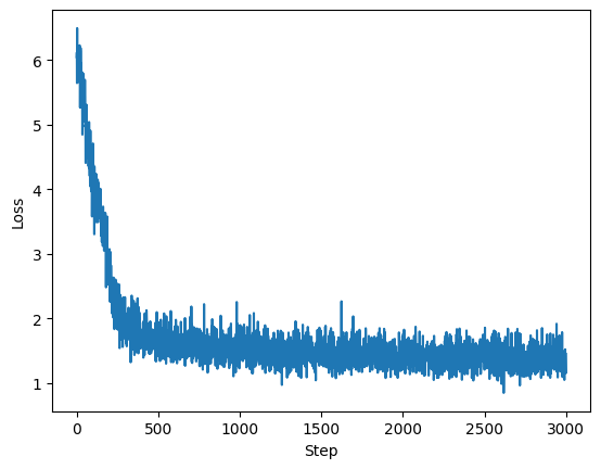
从上图我们可以看到 loss 明显下降，说明 CFGTrainer.get_train_loss 的训练流程是有效的，模型确实在学习条件向量场。

接下来我们来可视化训练结果：

#####################
# Visualize Results #
#####################

# User knobs
guidance_strength = 1.0 # try changing me!

fig, axes = plt.subplots(1, 3, figsize=(6 * 3, 6))

# Panel 1: Target
ax = axes[0]
x_data, _ = gmm.sample(250)
x_data = x_data.detach().cpu().numpy()
ax.scatter(x_data[:, 0], x_data[:, 1], s=5, marker="*")
ax.set_title("Target")

# Panel 2: Conditioned on each mode
ax = axes[1]
cfg_vector_field = CFGVectorFieldODE(vector_field, guidance_scale=guidance_strength, null_label=3)
simulator = EulerSimulator(cfg_vector_field)

batch_size = 250
labels = torch.arange(3).repeat_interleave(batch_size).to(device)
x_init = path.p_simple.sample(3 * batch_size) # b 2
ts = torch.linspace(0, 1, 100).expand(3 * batch_size, -1).to(device) # b nt
xs = simulator.simulate(x_init, ts, y=labels) # b 2
for idx in range(3):
    xs_idx = xs[idx * batch_size: (idx + 1) * batch_size].detach().cpu().numpy()
    ax.scatter(xs_idx[:, 0], xs_idx[:, 1], s=5, label=f"Mode {idx}", marker="*")
ax.legend()
ax.set_title(f"CFG w/ Guidance Strength {guidance_strength:.2f}")

# Panel 3: Unconditioned
ax = axes[2]
batch_size = 750
labels = torch.ones(batch_size).long().to(device) * 3
x_init = path.p_simple.sample(batch_size) # b 2
ts = torch.linspace(0, 1, 100).expand(batch_size, -1).to(device) # b nt
xs = simulator.simulate(x_init, ts, y=labels).detach().cpu().numpy() # b 2
ax.scatter(xs[:, 0], xs[:, 1], s=5, label=f"Mode {idx}", marker="*")
ax.set_title(f"Unguided Samples")

可视化结果如下：

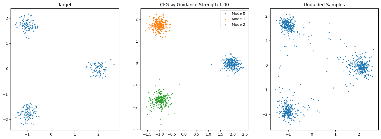
左侧 Target 图显示了真实 GMM 分布，三个模态清晰可见：

• Mode 0：右侧
• Mode 1：左上
• Mode 2：左下

这就是模型要学习的目标分布。

中间图 CFG w/ Guidance Strength 1.00 中，不同颜色对应不同条件标签。可以看到：

• Mode 0 的样本集中在右侧；
• Mode 1 的样本集中在左上；
• Mode 2 的样本集中在左下。

这说明模型确实学会了根据标签生成对应模态。也就是说：

$$u_t^{\theta }(x|0),u_t^{\theta }(x|1),u_t^{\theta }(x|2)$$

已经能够分别把初始高斯样本推到不同的 GMM 分量附近。

这证明 MLPConditionalVectorField.forward 中的标签 embedding 起作用了，模型不是无条件地生成任意模态，而是能按照标签控制输出。

右侧 Unguided Samples 图中，所有样本都使用 null label：

$$y=\varnothing$$

可以看到，它仍然生成了三个模态附近的点，而不是只生成某一个模态。

这说明模型在 label dropout 训练下，也学到了无条件分布：

$$p_{\text{data}}(x)$$

即三个高斯分量的混合分布。

不过无条件样本中间存在一些散点，这也比较正常，因为无条件模型需要同时覆盖所有模态，且 MLP 训练有限，ODE 积分也存在近似误差。

OK，这说明 sanity check 基本通过。

篇幅限制原因，Part 3、Part 4 以及 Part 5 的实现我们放在下篇文章中。