API

Rest风格API

文档地址

操作索引

基本概念

Elasticsearch是基于Lucence的全文检索，本质也是存储数据，很多概念与Mysql类似

对比关系：

索引(indices) ——>Databases数据库
类型(type)——>Table数据表
文档(Document)——>Row行
字段(Field)——>Columns列

Elasticsearch本身就是分布式的，因此即使只有一个节点，Elasticsearch默认也会对你的数据进行分片和副本操作，当你向集群添加新数据时，数据也会在新加入的节点中进行平衡；

创建索引

语法

Elasticsearch采用Rest风格API，所以其API就是一次请求，可以用任何工具发起http请求

创建索引的请求格式：

• 请求方式：PUT；
• 请求路径：/索引库名
• 请求参数：json格式

使用Kibana来操作

PUT westos
{
  "settings": {
    "number_of_shards": 1,
    "number_of_replicas": 1
  }
  
}

settings:索引库的设置

• number_of_shards:分片的数量
• number_of_replicas:副本数量，1表示没有副本

查看索引设置

使用get *可以查看所有索引库配置

删除索引

再次查看

也可以用HEAD请求查看索引是否存在

映射配置

再添加数据之前必须定义映射

什么是映射？

映射是定义文档的过程，文档包含哪些字段，这些字段是否保存，是否索引，是否分词等，只有配置清楚，Elasticsearch才会帮我们进行索引库的创建；

创建映射字段

• 类型名称goods：类似于数据库中的不同表字段名
• type：类型，可以是text，long，date，integer，object，数组等；
• index：是否索引，默认为true；
• store：是都存储，默认为false，不过在Elasticsearch中不管是true还是false都会存储，因为在Elasticsearch中不是由这个属性来控制的，而是_rouce
• analyzer:分词器，这里的ik_max_word即使用ik分词器；

查看映射关系

语法：

GET /索引库名/_mapping

字段属性详解

type

• String类型：

  • text：可分词，不可参与聚合；
  • keyword：不可分词，数据会作为完整字段进行匹配，可以参与聚合；

• Numerical数值类型：

  • 基本数据类型：long、interger、short、byte、double、float、half_float；
  • 浮点数的高精度类型：scaled_float
    • 需要指定一个精度因子，比如10或100。elasticsearch会把真实值乘以这个因子后存储，取出时再还原。

• Date：日期类型
  elasticsearch可以对日期格式化为字符串存储，但是建议我们存储为毫秒值，存储为long，节省空间。

index

• true：字段会被索引，则可以用来进行搜索，默认值就是true；
• false：字段不会被索引，不能用来搜索；

默认就是true，但有些字段我们不希望被索引，比如商品的图片信息，就需要手动设置为false；

store

是否将数据进行额外存储；

在Lucence和solr中，如果一个字段的store设置为false，那么在文档列表中就不会有这个字段的值，用户搜索结果中就不会显式出来；

但是在Elasticsearch中，即便是false，也可以搜索到结果；

原因是Elasticsearch在创建文档索引时，会将文档中的原始数据备份，保存到一个叫_source的属性中，而且我们可以通过滤_source来选择哪些要显示，哪些不显示；

而如果设置store为true，就会在_source以外额外存出一份数据，多余，因此一般都会将store设置为false，默认就是false；

新增数据

随机生成id

语法：

POST /索引库名、类型名
{
“key”:“value”
}

查看数据：

• _source:源文档信息，所有的数据都是在里面；
• _id：这条文档的唯一标识，与文档自己的id字段没有关联；

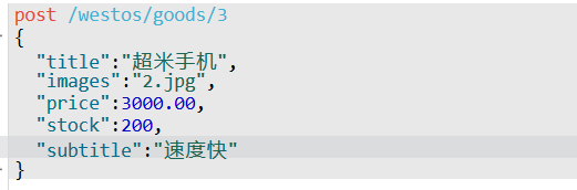
自定义id

语法：

POST /索引库名/类型/id值
{
}

智能判断

事实上，Elasticsearch非常智能，你不需要给索引库设置任何mapping映射，他可以根据你输入的数据来判断类型，动态添加数据映射；

指定两个没有定义的字段

查看映射

可以看到stock被映射成功了，而subtitle字符串类型映射出了两个值，一个是text，另一个是fields.keyword

如果想指定String类型映射类型，可以在设置映射时指定

修改数据

把刚才的请求方式改为PUT就是修改了，不过必须指定id，如果不指定就变成了新增

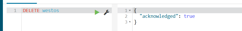
删除数据

删除使用DELETE请求，同样，需要根据id进行删除；

查询

从四块来讲:

• 基本查询；
• _source过滤；
• 结果过滤；
• 高级查询；
• 排序

基本查询

GET /索引库名/_search
{
	"query":{
				"查询类型":{
						"查询条件":"查询条件值"
				}
	}
}

这里的query代表一个查询对象，里面可以有不同的查询属性；

• 查询类型：match_all,match,term,range等。
• 查询条件：查询条件会根据类型不同，写法也有差异；

查询所有(match_all)

• query:代表查询对象；
• match_all:代表查询所有；

结果分析：

• took:查询花费的时间，单位是毫秒；
• time_out：是否超时；
• _shards:分片信息；
• hits：搜索结果总览对象；
  • _index:索引库名；
  • _type:文档类型；
  • _id:文档id
  • _score:文档得分；
  • _source:文档的源数据；

匹配查询(match)

or

在上面的案例中，不仅会查询到电视，而且与小米相关的都会查询到，多个词之间是or关系，所以只要含有小米的都能查到；

and

只有既包含小米，又包含电视的才能匹配到

既想包含那些可能相关的文档，同时又排除那些不太相关的

match查询支持minimun_should_match最小匹配参数，折让我们可以指定必须匹配的词项数用来表示一个文档是否相关，我们可以将其设置为某个数字，更常用的做法是将其设置为一个百分数，因为我们无法控制用户搜索时输入的单词数量：

本例中搜索语句可以分为3个词，如果使用and关系，则必须3个词都满足才会匹配到，这里采用了最小品牌数75%，那么就是能匹配到3*75%=2个词即可。

多字段查询

multi_match与match类似，不过它支持多个字段中查询：

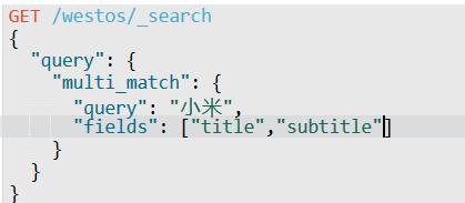
会在title和subtitle字段中查询这个词；

词条匹配(term)

term查询被用于精确值匹配，这些精确值可能是数字、时间、布尔或者那些未分词的字符串；

多词条精确匹配(terms)

结果过滤

默认情况下，Elasticsearch在搜索的结果中，会把文档中保存在_source的所有字段都返回，如果我们只想获取其中的部分字段，我们可以添加_source的过滤；

直接指定字段

指定includes和excludes

• includes：来指定想要显示的字段；
• excludes：来指定不想要的字段；

高级查询

布尔组合(bool)

bool把各种其它查询通过must(与)、must_not(非)、should(或)的方式进行组合

范围查询(range)

找出那些落在指定区间内的数字或者时间

模糊查询(fuzzy)

新增一条数据

POST /westos/goods/4
{
  "title":"apple手机",
  "images":"3.png",
  "price":6899.00
}

fuzzy和term查询的模糊等价，它允许用户搜索词条与实际词条的拼写出现偏差，但是偏差的编辑距离不得超过2；

可以通过fuzziness来指定允许的编辑距离：

GET /westos/_search
{
  "query": {
    "fuzzy": {
      "title": {
        "value": "appla",
        "fuzziness": 1
      }
    }
  }
}

过滤（filter）

条件查询中进行过滤

filter中还可以再次进行bool组合条件过滤

无查询条件，直接过滤

如果一次查询，只有过滤没有查询条件，不希望进行评分，可以使用constant_score取代只有filter语句的bool查询，在性能上是完全相同的，但对于提高查询简洁性和清晰度有很大的帮助；

排序

单字段排序

多字段排序

如果要结合使用price和_score进行查询，并且匹配的结果首先按照价格排序，然后按照的分排序：

集合aggregations

聚合可以让我们极其方便的实现对数据的统计、分析，实现这些统计功能比数据库方便的多，而且查询速度很快，可以实现实时搜索效果；

基本概念

Elasticsearch中的聚合，包含多种类型，最常用的是桶和度量；

桶
桶的作用，是按照某种方式对数据进行分组，每一组数据在ES中称为一个桶，例如我们根据国籍对人划分，可以得到中国桶、英国桶，日本桶……或者我们按照年龄段对人进行划分：0~10,10~20,20~30,30~40等。

Elasticsearch中提供的划分桶的方式有很多：

• Date Histogram Aggregation：根据日期阶梯分组，例如给定阶梯为周，会自动每周分为一组

• Histogram Aggregation：根据数值阶梯分组，与日期类似

• Terms Aggregation：根据词条内容分组，词条内容完全匹配的为一组

• Range Aggregation：数值和日期的范围分组，指定开始和结束，然后按段分组

• ……

综上所述，我们发现bucket aggregations 只负责对数据进行分组，并不进行计算，因此往往bucket中往往会嵌套另一种聚合：metrics aggregations即度量

度量

分组完成以后，我们一般会对组中的数据进行聚合运算，例如求平均值、最大、最小、求和等，这些在ES中称为度量

比较常用的一些度量聚合方式：

• Avg Aggregation：求平均值

• Max Aggregation：求最大值

• Min Aggregation：求最小值

• Percentiles Aggregation：求百分比

• Stats Aggregation：同时返回avg、max、min、sum、count等

• Sum Aggregation：求和

• Top hits Aggregation：求前几

• Value Count Aggregation：求总数

• ……

测试

插入新数据

PUT /cars
{
  "settings": {
    "number_of_shards": 1,
    "number_of_replicas": 0
  },
  "mappings": {
    "transactions":{
      "properties": {
        "color":{
          "type": "keyword"
        },
        "make":{
          "type": "keyword"
        }
      }
    }
  }
}

注意：在ES中，需要进行聚合、排序、过滤的字段其处理方式比较特殊，因此不能被分词，这里将color和make这两个文字类型的字段设置为keyword，这个类型不会被分词，将来就可以参与聚合；

导入数据

POST /cars/transactions/_bulk
{ "index": {}}
{ "price" : 10000, "color" : "red", "make" : "honda", "sold" : "2014-10-28" }
{ "index": {}}
{ "price" : 20000, "color" : "red", "make" : "honda", "sold" : "2014-11-05" }
{ "index": {}}
{ "price" : 30000, "color" : "green", "make" : "ford", "sold" : "2014-05-18" }
{ "index": {}}
{ "price" : 15000, "color" : "blue", "make" : "toyota", "sold" : "2014-07-02" }
{ "index": {}}
{ "price" : 12000, "color" : "green", "make" : "toyota", "sold" : "2014-08-19" }
{ "index": {}}
{ "price" : 20000, "color" : "red", "make" : "honda", "sold" : "2014-11-05" }
{ "index": {}}
{ "price" : 80000, "color" : "red", "make" : "bmw", "sold" : "2014-01-01" }
{ "index": {}}
{ "price" : 25000, "color" : "blue", "make" : "ford", "sold" : "2014-02-12" }

聚合为桶

按照汽车颜色来划分桶

GET /cars/_search
{
  "size": 0,
  "aggs": {
    "popular_colors": {
      "terms": {
        "field": "color"
      }
    }
  }
}

• size:查询条数，设置为0表示不关心搜索到的数据，只关心聚合结果；
• aggs：声明这是一个聚合查询，是aggregations的缩写
  • popular_colors:给这次聚合起一个名字：
    • terms：划分桶的方式，这里根据词条划分；
      • fields：划分桶字段

结果

{
  "took": 65,
  "timed_out": false,
  "_shards": {
    "total": 1,
    "successful": 1,
    "skipped": 0,
    "failed": 0
  },
  "hits": {
    "total": 8,
    "max_score": 0,
    "hits": []
  },
  "aggregations": {
    "popular_colors": {
      "doc_count_error_upper_bound": 0,
      "sum_other_doc_count": 0,
      "buckets": [
        {
          "key": "red",
          "doc_count": 4
        },
        {
          "key": "blue",
          "doc_count": 2
        },
        {
          "key": "green",
          "doc_count": 2
        }
      ]
    }
  }
}

• hits：查询结果为空，因为设置了size为0；
• aggregations：聚合的结果；
• popular_colors：定义的聚合的名称；
• buckets：查找到的桶，每个不同的color字段都会形成一个桶
  • key：这个桶对应的字段值；
  • doc_count:这个桶的文档数量；

桶内度量

我们需要告诉Elasticsearch使用哪个字段，使用何种度量方式进行运算，这些信息要嵌套在桶内，度量的运算会基于桶内的文档进行；

给刚才聚合结果添加求价格平均值的度量：

GET /cars/_search
{
  "size": 0,
  "aggs": {
    "popular_colors": {
      "terms": {
        "field": "color"
      },
      "aggs": {
        "avg_price": {
          "avg": {
            "field": "price"
          }
        }
      }
    }
  }
}

• aggs:在上一个aggs中添加新的aggs，可见度量也是一个聚合，度量是在桶内聚合；
• avg_price:聚合的名称；
• avg：度量的类型，这里是求平均值；
• field：度量运算的字段；

结果：

{
  "took": 161,
  "timed_out": false,
  "_shards": {
    "total": 1,
    "successful": 1,
    "skipped": 0,
    "failed": 0
  },
  "hits": {
    "total": 8,
    "max_score": 0,
    "hits": []
  },
  "aggregations": {
    "popular_colors": {
      "doc_count_error_upper_bound": 0,
      "sum_other_doc_count": 0,
      "buckets": [
        {
          "key": "red",
          "doc_count": 4,
          "avg_price": {
            "value": 32500
          }
        },
        {
          "key": "blue",
          "doc_count": 2,
          "avg_price": {
            "value": 20000
          }
        },
        {
          "key": "green",
          "doc_count": 2,
          "avg_price": {
            "value": 21000
          }
        }
      ]
    }
  }
}

桶内嵌套桶

事实上桶不仅可以嵌套运算，还可以再嵌套其他桶

比如：统计每种颜色的汽车，分别是那个制造商，再按make字段进行分桶：

GET /cars/_search
{
  "size": 0,
  "aggs": {
    "popular_colors": {
      "terms": {
        "field": "color"
      },
      "aggs": {
        "avg_price": {
          "avg": {
            "field": "price"
          }
        },
        "maker":{
          "terms": {
            "field": "make"
          }
        }
      }
    }
  }
}

结果：

{
  "took": 199,
  "timed_out": false,
  "_shards": {
    "total": 1,
    "successful": 1,
    "skipped": 0,
    "failed": 0
  },
  "hits": {
    "total": 8,
    "max_score": 0,
    "hits": []
  },
  "aggregations": {
    "popular_colors": {
      "doc_count_error_upper_bound": 0,
      "sum_other_doc_count": 0,
      "buckets": [
        {
          "key": "red",
          "doc_count": 4,
          "maker": {
            "doc_count_error_upper_bound": 0,
            "sum_other_doc_count": 0,
            "buckets": [
              {
                "key": "honda",
                "doc_count": 3
              },
              {
                "key": "bmw",
                "doc_count": 1
              }
            ]
          },
          "avg_price": {
            "value": 32500
          }
        },
        {
          "key": "blue",
          "doc_count": 2,
          "maker": {
            "doc_count_error_upper_bound": 0,
            "sum_other_doc_count": 0,
            "buckets": [
              {
                "key": "ford",
                "doc_count": 1
              },
              {
                "key": "toyota",
                "doc_count": 1
              }
            ]
          },
          "avg_price": {
            "value": 20000
          }
        },
        {
          "key": "green",
          "doc_count": 2,
          "maker": {
            "doc_count_error_upper_bound": 0,
            "sum_other_doc_count": 0,
            "buckets": [
              {
                "key": "ford",
                "doc_count": 1
              },
              {
                "key": "toyota",
                "doc_count": 1
              }
            ]
          },
          "avg_price": {
            "value": 21000
          }
        }
      ]
    }
  }
}

能读取到的信息：

• 红色车共有四辆；
• 红色车的平均售价是 $32，500 美元。
• 其中3辆是 Honda 本田制造，1辆是 BMW 宝马制造。

划分桶的其他方式

阶梯分桶Histogram

你只需要制定一个阶梯值来划分阶梯大小

比如：对汽车接个进行分组，阶梯值为10000：

GET /cars/_search
{
  "size": 0,
  "aggs": {
    "price": {
      "histogram": {
        "field": "price",
        "interval": 10000
      }
    }
  }
}

结果：

{
  "took": 18,
  "timed_out": false,
  "_shards": {
    "total": 1,
    "successful": 1,
    "skipped": 0,
    "failed": 0
  },
  "hits": {
    "total": 8,
    "max_score": 0,
    "hits": []
  },
  "aggregations": {
    "price": {
      "buckets": [
        {
          "key": 10000,
          "doc_count": 3
        },
        {
          "key": 20000,
          "doc_count": 3
        },
        {
          "key": 30000,
          "doc_count": 1
        },
        {
          "key": 40000,
          "doc_count": 0
        },
        {
          "key": 50000,
          "doc_count": 0
        },
        {
          "key": 60000,
          "doc_count": 0
        },
        {
          "key": 70000,
          "doc_count": 0
        },
        {
          "key": 80000,
          "doc_count": 1
        }
      ]
    }
  }
}

我们还可以使用min_doc_count参数为1来指定最少文档数量为1，过滤掉文档数量为0的桶

GET /cars/_search
{
  "size": 0,
  "aggs": {
    "price": {
      "histogram": {
        "field": "price",
        "interval": 10000,
        "min_doc_count": 1
      }
    }
  }
}

{
  "took": 11,
  "timed_out": false,
  "_shards": {
    "total": 1,
    "successful": 1,
    "skipped": 0,
    "failed": 0
  },
  "hits": {
    "total": 8,
    "max_score": 0,
    "hits": []
  },
  "aggregations": {
    "price": {
      "buckets": [
        {
          "key": 10000,
          "doc_count": 3
        },
        {
          "key": 20000,
          "doc_count": 3
        },
        {
          "key": 30000,
          "doc_count": 1
        },
        {
          "key": 80000,
          "doc_count": 1
        }
      ]
    }
  }
}

范围分桶

范围分桶与阶梯分桶类似，也是把数字按照阶段进行分组，只不过range方式需要你自己指定每一组的起始和结束大小。