Journey from Statistics to Machine Learning

     In recent times, machine learning (ML) and data science have gained popularity like never before. This field is expected to grow exponentially in the coming years. First of all, what is machine learning? And why does someone need to take pains to understand the principles? Well, we have the answers for you. One simple example could be book recommendations in e-commerce websites when someone went to search for a particular book or any other product recommendations which were bought together to provide an idea to users which they might like. Sounds magic, right? In fact, utilizing machine learning can achieve much more than this.

     Machine learning is a branch of study in which a model can learn automatically from the experiences based on data without exclusively being modeled like in statistical models. Over a period and with more data, model predictions will become better.

     In this first chapter, we will introduce the basic concepts which are necessary to understand statistical learning and create a foundation for full-time statisticians or software engineers who would like to understand the statistical workings behind the ML methods. 

Statistical terminology for model building and validation

Statistics is the branch of mathematics dealing with the collection, analysis, interpretation, presentation, and organization of numerical data.

Statistics are mainly classified into two subbranches:

• Descriptive statistics: These are used to summarize data, such as the mean, standard deviation for continuous data types (such as age, house price), whereas frequency and percentage are useful for categorical data (such as gender).
  unordered categorical (nominal, e.g. t-shirt color as a nominal feature ), and
  ordered categorical (ordinal, e.g. t-shirt size would be an ordinal feature, because we can define an order XL > L > M)
  cp14_2_Layers_config_numeric_continuou_Feature Column_boosted tree_n_batches_per_layer_repeat_estima_Linli522362242的专栏-CSDN博客
• Inferential statistics: Many times, a collection of the entire data (also known as population in statistical methodology[ˌmeθəˈdɑːlədʒi]方法学，方法论) is impossible, hence a subset of the data points is collected, also called a sample, and conclusions about the entire population will be drawn, which is known as inferential statistics. Inferences are drawn using hypothesis testing, the estimation of numerical characteristics, the correlation of relationships within data, and so on.

Statistical modeling is applying statistics on data to find underlying hidden relationships by analyzing the significance of the variables.

Machine learning

     Machine learning is the branch of computer science that utilizes past experience to learn from and use its knowledge to make future decisions. Machine learning is at the intersection of computer science, engineering, and statistics. The goal of machine learning is to generalize a detectable pattern or to create an unknown rule from given examples. An overview of machine learning landscape is as follows:

     Machine learning is broadly classified into three categories but nonetheless[ˌnʌnðəˈles]虽然如此, based on the situation, these categories can be combined to achieve the desired results for particular applications:

• Supervised learning: This is teaching machines to learn the relationship between other variables and a target variable, similar to the way in which a teacher provides feedback to students on their performance. The major segments within supervised learning are as follows:
  • Classification problem
  • Regression problem
• Unsupervised learning: In unsupervised learning, algorithms learn by themselves without any supervision or without any target variable provided. It is a question of finding hidden patterns and relations in the given data. The categories in unsupervised learning are as follows:
  • Dimensionality reduction
  • Clustering
• Reinforcement learning: This allows the machine or agent to learn its behavior based on feedback from the environment. In reinforcement learning, the agent takes a series of decisive actions without supervision and, in the end, a reward will be given, either +1 or -1. Based on the final payoff/reward, the agent reevaluates its paths. Reinforcement learning problems are closer to the artificial intelligence methodology rather than frequently used machine learning algorithms.
  
  What type of Machine Learning algorithm would you use to allow a robot to walk in various unknown terrains(地形)?
  
       Ans: Reinforcement Learning is likely to perform best if we want a robot to  learn to walk in various unknown terrains since this is typically the type of problem as a supervised or semisupervised learning problem, but it would be less natural.(Reinforcement Learning system called an agent in the context, can observe the environment, select and perform actions, and get rewards in return or penalities in the form of negative rewards. It must then learn by itself what is the best strategy, called a policy to get the most reward over time. A policy defines what action the agent should choose when it is in given situation)
  

     In some cases, we initially perform unsupervised learning to reduce the dimensions followed by supervised learning when the number of variables is very high. Similarly, in some artificial intelligence applications, supervised learning combined with reinforcement learning could be utilized for solving a problem; an example is self-driving cars in which, initially, images are converted to some numeric format using supervised learning and combined with driving actions (left, forward, right, and backward).

Statistical fundamentals and terminology for model building and validation

     Statistics itself is a vast subject on which a complete book could be written; however, here the attempt is to focus on key concepts that are very much necessary with respect to the machine learning perspective. In this section, a few fundamentals are covered and the remaining concepts will be covered in later chapters wherever it is necessary to understand the statistical equivalents of machine learning.

     Predictive analytics depends on one major assumption: that history repeats itself!

     By fitting a predictive model on historical data after validating key measures, the same model will be utilized for predicting future events based on the same explanatory variables(predictor variables or independent variables) that were significant on past data.
########################
     In regression analysis, we are given a number of predictor (explanatory) variables and a continuous response variable (outcome), and we try to find a relationship between those variables that allows us to predict an outcome.

     Note that in the field of machine learning, the predictor variables are commonly called "features," and the response variables are usually referred to as "target variables." We will adopt these conventions throughout this book.

     In machine learning and deep learning applications, we can encounter various different types of features: continuous, unordered categorical (nominal), and ordered categorical (ordinal). You will recall that in In machine learning and deep learning applications, we can encounter various different types of features: continuous(e.g. house price), unordered categorical (nominal, e.g. t-shirt color as a nominal feature ), and ordered categorical (ordinal, e.g. t-shirt size would be an ordinal feature, because we can define an order XL > L > M). You will recall that in cp4 Training Sets Preprocessing_StringIO_dropna_categorical_feature_Encode_Scale_L1_L2_bbox_to_anchor https://blog.csdn.net/Linli522362242/article/details/108230328, we covered different types of features and learned how to handle each type. Note that while numeric data can be either continuous or discrete, in the context of the TensorFlow API, "numeric" data specifically refers to continuous data of the floating point type.
######################## cp14_2_Layers_config_numeric_continuou_Feature Column_boosted tree_n_batches_per_layer_repeat_estima_Linli522362242的专栏-CSDN博客

     The first movers of statistical model implementers were the banking and pharmaceutical[ˌfɑːməˈsuːtɪkl; ˌfɑːməˈsjuːtɪkl]制药（学）的 industries; over a period, analytics expanded to other industries as well.

     Statistical models are a class of mathematical models that are usually specified by mathematical equations that relate one or more variables to approximate reality. Assumptions embodied by statistical models describe a set of probability distributions, which distinguishes it from non-statistical, mathematical, or machine learning models

     Statistical models always start with some underlying assumptions for which all the variables should hold, then the performance provided by the model is statistically significant. Hence, knowing the various bits and pieces involved in all building blocks provides a strong foundation for being a successful statistician.

In the following section, we have described various fundamentals with relevant codes:

• Population: This is the totality, the complete list of observations, or all the data points about the subject under study.
• Sample: A sample is a subset of a population, usually a small portion of the population that is being analyzed.

Usually, it is expensive to perform an analysis of an entire population; hence, most statistical methods are about drawing conclusions about a population by analyzing a sample.

• Parameter versus statistic: Any measure that is calculated on the population is a parameter, whereas on a sample it is called a statistic.
• Mean: This is a simple arithmetic average, which is computed by taking the aggregated sum of values divided by a count of those values. The mean is sensitive to outliers in the data. An outlier is the value of a set or column that is highly deviant from the many other values in the same data; it usually has very high or low values.
• Median(==Q2, the second quartile): This is the midpoint of the data, and is calculated by either arranging it in ascending or descending order. If there are N observations.
  Application: Binary search or students' score(if the average(mean)>60, and your professor want at least half of students pass the course, but if your professor use the mean as measure, then most number of students will fail since few students got very high score and the mean is affected by the high scores(this means the average will not reflect the “typically” student scores), so he will consider to use the median of the scores as measure)
  
  Find the median of a batch of n numbers is easy as long as you remember to order the values first.
  If n is odd, the median is the middle value. Counting in from the ends, we find the value in the (n+1)/2 position
  if n is even, there are two middle values. So, in the case, the median is the average of the two values in positions n/2 and n/2+1
  
  Example: The U.S. Census[ˈsensəs]统计 Bureau[ˈbjʊərəʊ]局 reports the median family income in its summary of census data. Why do you suppose they use the median instead of the mean? What might be the disadvantages of reporting the mean?
       Incomes are probably skewed to the right, making the median more appropriate to measure distribution center. The mean will be affected by the high end of family incomes and would not reflect the “typically” family incomes as well as the median would.
  
• Mode(众数): This is the most repetitive data point in the data: the most frequent number!
• (symmetrical distribution VS asymmetrical distribution)

The Python code for the calculation of mean, median, and mode using a numpyarray and the stats package is as follows:

import numpy as np
from scipy import stats

data = np.array([4,5,1,2,7,2,6,9,3])

# Calculate Mean

dt_mean = np.mean(data);
print("Mean :", round(dt_mean,2))

# Calculate Median

dt_median = np.median(data);
print("Median :", dt_median)

# Calculate Mode :  This is the most repetitive data point in the data: the most frequent number!

dt_mode = stats.mode(data);
print("Mode :", dt_mode[0][0]) # [0]:first element in ModeResult, 
                               # [0][0]: first value in mode list((the most frequent number)

dt_mode

 

#######################################################

a = np.array([[2, 2, 2, 1],
              [1, 2, 2, 2],
              [1, 1, 3, 3]])
print("# Print mode(a):", stats.mode(a)) # in each column
print("# Print mode(a.transpose()):", stats.mode(a.transpose())) # in each row
                                                            
print("# a的每一列中最常见的成员为：{}，分别出现了{}次。".format(stats.mode(a)[0][0], stats.mode(a)[1][0])) # in each column
print("# a的第一列中最常见的成员为：{}，出现了{}次。".format(stats.mode(a)[0][0][0], stats.mode(a)[1][0][0])) # 1 in the first column
print("# a的每一行中最常见的成员为：{}，分别出现了{}次。".format(stats.mode(a.transpose())[0][0], stats.mode(a.transpose())[1][0])) # in each row
print("# a中最常见的成员为：{}，出现了{}次。".format(stats.mode(a.reshape(-1))[0][0], stats.mode(a.reshape(-1))[1][0]))

print("# a的第一列中最常见的成员为：{}，出现了{}次。".format(stats.mode(a)[0][0][0], stats.mode(a)[1][0][0]))
print("# a的每一行中最常见的成员为：{}，分别出现了{}次。".format(stats.mode(a.transpose())[0][0], stats.mode(a.transpose())[1][0]))
print("# a中最常见的成员为：{}，出现了{}次。".format(stats.mode(a.reshape(-1))[0][0], stats.mode(a.reshape(-1))[1][0]))

for example 2,1,1 

Where mode is calculated simply the number of observations in a data set which is occurring most of the time.   

First the modal group with the highest frequency needs to identify If the interval is not continuous 0.5 should be subtracted from the lower limit Mode and 0.5 should be added from the upper limit Mode.

The (h) is Called the Size of the class interval is 1= 1.5-0.5 or 2.5-1.5

1 (frequency=2) : [1-0.5, 1+0.5] = [0.5, 1.5]
2 (frequency=1) : [2-0.5, 2+0.5] = [1.5, 2.5]

mode=E5 + E4*(E2-E1)/((E2-E1)+(E2-E3))  =1  and we just use the integer so we drop the decimal 

<==

Mode Formula | Calculator (Examples with Excel Template)

Mode Formula – Example #1

Where mode is calculated simply the number of observations in a data set which is occurring most of the time.

Mode Formula – Example #2  : Modal Group Which is Most Frequent i.e 60.5-65.5 ? : 61.5

==>

Note: 

• First the modal group with the highest frequency needs to identify If the interval is not continuous 0.5 should be subtracted from the lower limit Mode and 0.5 should be added from the upper limit Mode. Then the interval will be
• Then the lower frequency is of the modal group which is 4, in this case, is taken as fm+1 and
• fm-1 will become 7 in this example. And we have fm that is the frequency as 8.
• The (h) is Called the Size of the class interval is 5 which we have considering the starting interval as well. L is 60.5.

Mode Formula – Example #3

     The following are the distributions of heights in a certain class of students in a certain Mode

Calculate the Mode by using the Given Information.

==>

Solution:

• If the interval is not continuous 0.5 should be subtracted from the lower limit Mode and 0.5 should be added from the upper limit Mode.
• Then the interval(h) will be 3

Modal Group Which is Most Frequent i.e 165.5-168.5 : 167.35

########################################################

     We have used a NumPy array instead of a basic list as the data structure; the reason behind using this is the scikit-learn package built on top of NumPy array in which all statistical models and machine learning algorithms have been built on NumPy array itself. The mode function is not implemented in the numpy package, hence we have used SciPy's stats package. SciPy is also built on top of NumPy arrays.

• Measure of variation:
       Dispersion is the variation in the data, and measures the inconsistencies in the value of variables in the data. Dispersion actually provides an idea about the spread rather than central values.
   
• Range: This is the difference between the maximum and minimum of the value.
   
• Variance:
       This is the mean of squared deviations from the mean (xi = data points, µ = mean of the data, N = number of data points). The dimension of variance is the square of the actual values. The reason to use denominator N-1 for a sample instead of N in the population is due the degree of freedom. 1 degree of freedom lost in a sample by the time of calculating variance is due to extraction of substitution of sample: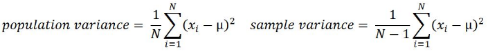
  
  
• Standard deviation:
       This is the square root of variance. By applying the square root on variance, we measure the dispersion with respect to the original variable rather than square of the dimension:
  
  
   
  Boxplot: 
  
• The box represents quartiles of the data方框代表数据的四分位数,
• Quantiles:
       These are simply identical fragments of the data. Quantiles cover percentiles, deciles, quartiles, and so on. These measures are calculated after arranging the data in ascending order:
  • Percentile: This is nothing but the percentage of data points below the value of the original whole data. The median(the center line denotes the median value) is the 50th percentile, as the number of data points below the median is about 50 percent of the data.
  • Decile: This is 10th percentile, which means the number of data points below the decile is 10 percent of the whole data.
  • Quartile: This is one-fourth of the data, and also is the 25th percentile. The first quartile is 25 percent of the data, the second quartile is 50 percent of the data, the third quartile is 75 percent of the data. The second quartile is also known as the median or 50th percentile or 5th decile.
  • Interquartile range( IQR = Q3-Q1 ): This is the difference between the third quartile(Q3, upper quartile) and first quartile(Q1, lower quartile). It is effective in identifying outliers in data. The interquartile range describes the middle 50 percent of the data points
  • Outliers (the abnormal point, ): <Q1-1.5*IQR or >Q3+1.5*IQR
  • Upper Quartile (上边缘, Q3) ：The maximum value in the data other than the abnormal point
  • Lower Quartile (下边缘, Q1) ：The minimum value in the data other than the abnormal point
     
  • the whiskers represent the full range of the data
     
  • n=40 numbers: 53 53 61 61 63 65 67 67 69 69, 69 70 70 71 74 75 75 76 77 78, 79 80 81 81 81 81 82 84 85 86, 87 87 87 88 89 90 91 91 94 95
    Q1=(69+69)/2=69；Q3=(86+87)/2=86.5, since n is  even.
    IQR = Q3-Q1=86.5-69=17.5；
    lower fence: Q1－1.5IQR=42.75；
    upper fence: Q3 + 1.5IQR=112.75；So there are no outliers。
  • upper marginal : 95，lower marginal: 52

The Python code is as follows:

import numpy as np
from statistics import variance, stdev

game_points = np.array( [35,56,43,59,63,79,35,41,64,43,93,60,77,24,82], 
                        dtype=float
                      )

# Calculate Variance

dt_var = variance(game_points)
print( "Sample variance:", round(dt_var,2) ) 

 

# Calculate Standard Deviation

dt_std = stdev(game_points)
print( "Sample std.dev:", round(dt_std,2) ) 

# Calculate Range 

dt_rng = np.max(game_points, axis=0) - np.min(game_points, axis=0)
print( "Range:",dt_rng ) 

 

#Calculate percentiles 

print ("Quantiles:") 
for val in [20,80,100]: 
  dt_qntls = np.percentile( game_points, val )  
  print( str(val) + "%", round(dt_qntls, 1) ) 

 

# Calculate IQR (Interquartile range)

q75, q25 = np.percentile( game_points, [75 ,25] )
print ( "Inter quartile range:",q75-q25 )

 

• Hypothesis testing: This is the process of making inferences about the overall population by conducting some statistical tests on a sample. Null and alternate hypotheses are ways to validate whether an assumption is statistically significant or not.
  
  Parameter versus statistic: Any measure that is calculated on the population is a parameter, whereas on a sample it is called a statistic.
  Null Hypothesis  is the claim about a population parameter that the researcher wants to test OR Null Hypothesis   is a statement that the value of a population parameter is equal to some claimed value.
  Alternative Hypothesis (OR ) is the the opposite of , representing the values of a population aparameter for which the research wants to gather evidence to support.
  1.请写出下列论断的零假设与备择假设
  （1）百事可乐公司声称，其生产的罐装可乐的标准差为0.005磅 :  
  （2）某社会调查员说从某项调查得知中国的离婚率高达38.5% : 
  （3）某学校招生宣传手册中写道，该学校的学生就业率高达99%。
  OR
  someone claims : the mean monthly cell phone bill of the nyc is $75 :  vs 
  someone claims : the proportion of adults in the nyc with cell phones is 0.9 : vs
   
• P-value（Rejection Region Area, 拒绝域的面积）: The probability of obtaining a test statistic result is at least as extreme as the one that was actually observed( the probability we obstain a more extreme value than the observed test statistic Z. 当原假设为真时,所得到的样本观察结果或更极端结果出现的概率), assuming that the null hypothesis is true (usually in modeling, against each independent variable, a p-value < 0.05 is considered significant and > 0.05 is considered insignificant; nonetheless, these values and definitions may change with respect to context).
  
  当p-值足够小时，即小于置信水平 ( assuming that the null hypothesis is true, the probability of the test statistic Z in the Rejection Region)时，我们可以拒绝零假设。
• 

• The steps involved in hypothesis testing are as follows:

• 1. Assume a null hypothesis (usually no difference, no significance, and so on; a null hypothesis always tries to assume that there is no anomaly pattern and is always homogeneous同类的, and so on).
     OR
     State null hypothesis  and alternative hypothesis 
     Check assumptions made about population.
  2. Collect the sample.
  3. Calculate test statistics from the sample in order to verify whether the hypothesis is statistically significant or not.
     OR
     Calculate test statistic from a sample to measure the evidence that goes against与...相悖 .
  4. Decide either to accept or reject the null hypothesis based on the test statistic.
     OR
     Determine rejection region (R), where we believe the evidence is sufficient to reject.
     then see whether the test statistic falls in the rejection region and then draw conclusion.
• Example of hypothesis testing: A chocolate manufacturer who is also your friend claims that all chocolates produced from his factory weight at least 1,000 g and you have got a funny feeling that it might not be true; you both collected a sample of 30 chocolates and found that the average chocolate weight as 990 g with sample standard deviation as 12.5 g. Given the 0.05 significance level , can we reject the claim made by your friend?
  
  Unknown:population variance or polulation standard deviation 
  but, known:sample standard deviation  ==> 
  
  The null hypothesis :  µ0 ≥ 1000 (all chocolates weigh more than 1,000 g ==> we only consider one tail area==>)
  （if your friend claims that all chocolates produced from his factory weigh is 1,000 g,
     then The null hypothesis :  µ0 = 1000, V.S  µ0 1000
     ... ...
   Critical t value(临界 t 值, , n-1) from t tables  
  ）
  
  Collected sample: 
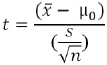
  Calculate test statistic from the sample:  (使用的是临界值(critical value)法)
  
                                                                    t = (990 - 1000) / (12.5/sqrt(30)) = 一 4.3818     (use left tail一 the rejection Region)
  df=n-1=30-1=29 : df tells you which row the the t-talbe to use
   ==>
  
  Critical t value(临界 t 值, , n-1) from t tables = t[0.05, 30-1] = 1.699 ==>(use left tail一 the rejection space)==> - t_a=一 t[0.05, 30-1]= 一1.699 > 一4.3818        (included)     (t: horizontal axis maximum)
  
  
  P-value = 7.03 e-05      Note:    we can't not get this value from the t table, but we know the P-value in the rejection Region is << 0.05 
  当p-值足够小时，即小于置信水平 ( assuming that the null hypothesis is true, the probability of the test statistic in the Rejection Region)时，我们可以拒绝零假设。
  
  
  
  Conclusion:
  Test statistic is -4.3818, which is less than the critical value of -1.699. Hence, we can reject the null hypothesis (your friend's claim that all chocolates produced from his factory weigh at least 1,000 g) that the mean weight of a chocolate is above 1,000 g.
  
  Also, another way of deciding the claim is by using the p-value. A p-value less than 0.05 means both claimed values and distribution mean values are significantly different, hence we can reject the null hypothesis: ​​​​​​

The Python code is as follows:

from scipy import stats
import numpy as np

xbar = 990
mu0 = 1000 #population's mean
s=12.5     #standard deviation
n=30

# Test Statistic(from the sample)

t_sample = (xbar - mu0) / ( s/np.sqrt(float(n)) )
print("Test Statistic: ", round(t_sample,2))

 
# Critical value from t-table

alpha = 0.05
t_alpha = stats.t.ppf(alpha, n-1)
print( "Critical value from t-table: ", round(t_alpha, 3) )

 
# Lower tail p-value from t-table:                        # stats.t.sf : Survival function (1 - cdf) at x of the given RV.

p_val = stats.t.sf( np.abs(t_sample), n-1 )
print( "Lower tail p-value from t-table: ", p_val )

• Type I and II error: Hypothesis testing is usually done on the samples rather than the entire population, due to the practical constraints of available resources to collect all the available data. However, performing inferences about the population from samples comes with its own costs, such as rejecting good results or accepting false results, not to mention separately, when increases in sample size lead to minimizing type I and II errors:
  vs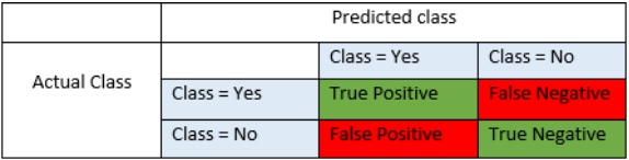
  

  Type I error: Rejecting a null hypothesiswhen it is true, (OR  is true, but we reject it by mistake. Because we mistakenly think is False, P=target class(the null hypothesis=False, Reject) )
  α = probability of a Type I error, known as a "false positive"(FP)
  1-α = probability of a "true negative"(TN), i.e., correctly not rejecting the null hypothesis, since =True, non-false

  Type II error: Accepting a null hypothesiswhen it is false, (OR  is false, but we fail to reject it.)
  β = probability of a Type II error, known as a "false negative"(FN) ( Because we mistakenly think is True, N=non-target class(the null hypothesis=True, Accept))
  1-β = probability of a "true positive"(TP), i.e., correctly rejecting the null since=False

  T: True prediction or classify correctly;     F: False prediction or classify incorrectly
  P: instance is truely belong to target class(the null hypothesis=False, Reject) based on the fact;     
  N: instance is not belong to target class(the null hypothesis=True, Accept) based on the fact
  Accuracy = (TP+TN)/(TP+FP+FN+TN)
  Precision = TP/(TP+FP) # True predicted/ (True predicted + False predicted)
  Recall = TP/(TP+FN)
  https://blog.csdn.net/Linli522362242/article/details/103786116

       The statistical power of a binary hypothesis test is the probability that the test correctly rejects the null hypothesis () when a specific alternative hypothesis () is true(since=False, reject). It is commonly denoted by (1-β = probability of a "true positive"(TP), i.e., correctly rejecting the null since=False), and represents the chances of a "true positive"(TP) detection conditional on the actual existence of an effect to detect. Statistical power ranges from 0 to 1, and as the power of a test increases(1-β), the probabilityof making a type II error by wrongly failing to reject the null hypothesis decreases. 
  β = probability of a Type II error, known as a "false negative"(FN) ( Because we mistakenly think is True, N=non-target class(the null hypothesis=True, Accept))

• To measure the likelihood of making Type I or II error, we define: 
  
  α = probability of a Type I error, known as a "false positive"(FP)
  β = probability of a Type II error, known as a "false negative"(FN) ( Because we mistakenly think is True, N=non-target class(the null hypothesis=True, Accept))
  
  Ideally, we want both α and to β be small. However, if we decrease α, we increase β, and vice-versa.
  We will make α small(increase 1-α, TP):
       If we reject , since we're pretty sure it's false(increase 1-α, TP);
       we will fail to reject , we don't claim  is true because we may have a big chance(large β) to make Type II error when =True base on the fact.

• Normal distribution: This is very important in statistics because of the central limit theorem, which states that the population of all possible samples of size n from a population with mean μ and variance  approaches a normal distribution:

  
  
  Example: Assume that the test scores of an entrance exam fit a normal distribution. Furthermore, the mean test score is 52 and the standard deviation is 16.3. What is the percentage of students scoring 67 or more in the exam?
  ==>
  
  ( hidden: (67-52)/16.3=0.92)
  

  The Python code is as follows:

  from scipy import stats
  
  xbar=67
  mu0=52
  s=16.3
  
  # Calculating z-score
  z = (xbar-mu0)/s # z = (67-52)/16.3
  
  # Calculating probability under the curve
  p_val = 1 - stats.norm.cdf(z)
  print( "Prob. to score more than 67 is", round(p_val*100, 2), "%" )

  

• A supervisor of a large company believes that on the average it takes a worker 2 minutes to complete a particular task with standard deviation of 0.2. Suppose the avereage time for 100 randomly selected workers to complete that task is 2.06 minutes. Is the supervisor's claim correct? Use =0.05.
  
  known:population variance  ==>  ==>
  
       : μ=2  vs   : μ !=2
       Calculate test statistic >1.96 in the right Rejection Region
       We know =0.05 and  (hidden: 1-0.025=0.975 ~=1.96)
  STANDARD NORMAL DISTRIBUTION: Table Values Represent AREA(1- for 1 tail) to the LEFT of the Z score.
  
    https://www.math.arizona.edu/~rsims/ma464/standardnormaltable.pdf
   R: Rejection Region
  
  The supervisior's claim is false and the mean time to complete the task is more than 2 mins.
• Connection to Confidence Interval
  We can also test  under  significance level using 100*(1-)% Confidence Interval
  
   We know =0.05 and  (hidden: 1-0.025=0.975 ~=1.96)
  
  
  ########################
  
   is significance level置信水平(the probability of the test statistic Z in the Rejection Region), ( Z=2.12 ==> =0.983 ==>the smallest =0.017 called P-value)
  当p-值足够小时，即小于置信水平 (the probability of the test statistic Z in the Rejection Region)时，我们可以拒绝零假设。
• 
  =0.95 Confidence Interval置信区间
   
   
  (P-value=0.017 <, in the Rejection Region) 
  
  
  (P-value=0.017 >, not in the Rejection Region)2.12 not in the Rejection Region
  
  What is the samllest  that we can choose if we want to reject ?
  Z=2.12 ==> =0.983 ==> >=0.017 ==> 
  
  Observed significance Level: p-Value
  p-value is the probability we obstain a more extreme value than the observed test statistic.(The probability of obtaining a test statistic result is at least as extreme as the one that was actually observed)
  
  
• Chi-square, also written as test:
  
       This test of independence is one of the most basic and common hypothesis tests in the statistical analysis of categorical data. Given two categorical random variables X and Y, the chi-square test of independence determines whether or not there exists a statistical dependence between them.
  
       The test is usually performed by calculating χ2 from the data and χ2 with (m-1, n-1) degrees from the table. A decision is made as to whether both variables are independent based on the actual value and table value, whichever is higher: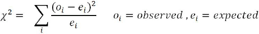
  
  Example: In the following table, calculate whether the smoking habit has an impact on exercise behavior:
  

  import pandas as pd
  from scipy import stats
  
  survey = pd.read_csv("/content/drive/MyDrive/Numerical Computing/dataset/survey.csv")
  survey.head(n=10)

  

  # Tabulating 2 variables with row & column variables respectively
  # Compute a simple cross tabulation简单交叉表 of two (or more) factors. 
  # By default computes a frequency table of the factors 
  # unless an array of values and an aggregation function are passed.
                          # If margins is True, will also normalize margin values.
  survey_tab = pd.crosstab( survey.Smoke, survey.Exer, margins=True )
  survey_tab

  
  While creating a table using the crosstab function, we will obtain both row(survey.Smoke) and column(survey.Exer) totals field extra(All). However, in order to create the observed table, we need to extract the variables part and ignore the totals:
  # Creating observed table for analysis

  observed = survey_tab.iloc[0:4, 0:3]
  observed

   
       The degrees of freedom(df): (num_rows - 1) * ( num_columns - 1)=(4-1)*(3-1)=3*2= 6
       The chi2_contingency function in the stats package uses the observed table and subsequently calculates its expected table, followed by calculating the p-value in order to check whether two variables are dependent or not.
  If p-value < 0.05 (), there is a strong dependency between two variables , whereas
  if p-value > 0.05(), there is no dependency between the variables:

  contg = stats.chi2_contingency( observed=observed )
  # return
  # chi2 : float
  #     The test statistic.
  # p : float
  #     The p-value of the test
  # dof : int
  #     Degrees of freedom
  # expected : ndarray, same shape as observed
  #     The expected frequencies, based on the marginal sums of the table.
  contg

   <== 11*98/236=4.56779661 <==<==
  # Find the expected values: 

  pd.DataFrame(contg[3], dtype=float)

   ==> ==>The test statistic : 5.488545890584232

  p_value = round(contg[1],3)
  print("P-value is: ", p_value)

    The p-value is 0.483 > 0.05, which means there is no dependency between the smoking habit and exercise behavior.
  OR Check X table [df=6, =0.05]==>14.067> 5.488545890584232 ==> P-value = P( > 5.488545890584232 ) ==> the test statistic is not falls in the rejection region, so we cannot reject  (OR there is no dependency between the variables)

• *********************************************************************************************************
  

• *********************************************************************************************************
  
  
  *********************************************************************************************************
• ANOVA:
  
       Analyzing variance tests the hypothesis that the means of two or more populations are equal. ANOVAs assess the importance of one or more factors by comparing the response variable(target variable) means at the different factor levels. The null hypothesis states that all population means are equal while the alternative hypothesis states that at least one is different.
  
   

  • Example: A fertilizer[ˈfɜːrtəlaɪzər]肥料 company developed three new types of universal fertilizers after research that can be utilized to grow any type of crop. In order to find out whether all three have a similar crop yield产量, they randomly chose six crop types in the study. In accordance with the randomized block design, each crop type will be tested with all three types of fertilizer separately. The following table represents the yield in . At the 0.05 level of significance, test whether the mean yields for the three new types of fertilizers are all equal:
    
    
    The Python code is as follows:

    import pandas as pd
    from scipy import stats
    
    fetilizers = pd.read_csv( "/content/drive/MyDrive/Numerical Computing/dataset/fetilizers.csv")
    fetilizers

    # 6 crop types
    Calculating one-way ANOVA using the stats package:
    ################################Business Statistics (2nd Edition) - 道客巴巴 Page: 760, 729
    stats.f_oneway : 
         Perform one-way ANOVA.

         The one-way ANOVA tests the null hypothesis that two or more groups have the same population mean. The test is applied to samples from two or more groups, possibly with differing sizes.
    
    Parameters
         sample1, sample2, ... : array_like
             The sample measurements for each group.
    
    Returns
         statistic : float
            The computed F statistic of the test.
         pvalue : float
         The associated p-value from the F distribution.
    
    Notes
    The ANOVA test has important assumptions that must be satisfied in order for the associated p-value to be valid.

    The samples are independent.
    Each sample is from a normally distributed population.
    The population standard deviations of the groups are all equal. This property is known as homoscedasticity[ˈhoʊməsɪdæsˈtɪsəti]同方差性，[数] 方差齐性.
    ################################

  • one_way_anova = stats.f_oneway( fetilizers["fertilizer1"], fetilizers["fertilizer2"], fetilizers.fertilizer3 )
    one_way_anova

    

    print("statistic: ", round( one_way_anova[0], 2 ), 
          ", p-value:", round(one_way_anova[1], 3) 
         )

    
         Result: The p-value did come as greater than 0.05, hence we cannot reject the null hypothesis that the mean crop yields of the fertilizers are equal. Fertilizers make a insignificant difference to crops.
    
    Note: sample variance : vs 

    ( (7-5.5)**2 + (3-5.5)**2 + (6-5.5)**2 + (6-5.5)**2 )/(4-1)

    

    ( (6-6)**2 + (5-6)**2 + (5-6)**2 + (8-6)**2 )/(4-1)

     
    

• 
• Confusion matrix: This is the matrix of the actual versus the predicted. This concept is better explained with the example of cancer prediction using the model:
• *********************************************************************************************************
• *******************************************************************************************************************************************
• 
• 
• 

• 
• 
• ************************************************************************************************************************
• ********************************************************************************************************************
• 
• 
  
• 
• 
• 
• *********************************************************************************************************
• 
• 

1-0.9991=0.0009 < alpha=0.05

************************************************************************************************************************

use t table with two tails

************************************************************************************************************************

• 
• ************************************************************************************************************************
• •