
【第十四周】Jupyter作业
题目来源:https://nbviewer.jupyter.org/github/schmit/cme193-ipython-notebooks-lecture/blob/master/Exercises.ipynb
·
题目来源:
https://nbviewer.jupyter.org/github/schmit/cme193-ipython-notebooks-lecture/blob/master/Exercises.ipynb

see Note in part 2
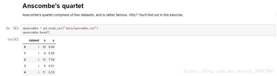
(1)Compute the mean and variance of both x and y
print( 'The average of x is {:.2f}'.format(anascombe['x'].mean()))
print( 'The average of y is {:.2f}'.format(anascombe['y'].mean()))
print( 'The variance of  x is {:.2f}'.format(anascombe['x'].var()))
print( 'The variance of  y is {:.2f}'.format(anascombe['y'].var()))
结果:

(2)Compute the correlation coefficient between x and y
a=np.array([anascombe['x'],anascombe['y']])
b= np.corrcoef(a)
print(b[0][1])
结果:

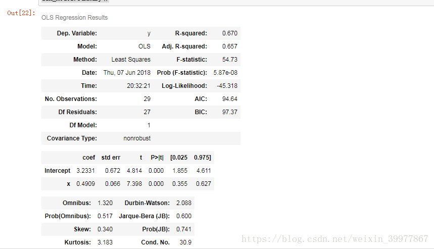
(3)Compute the liner regression line(hint:use statsmodels and look at the Statsmodels notebook)
n = len(anascombe)
is_train = np.random.rand(n) < 0.7
train = anascombe[is_train].reset_index(drop=True)
test = anascombe[~is_train].reset_index(drop=True)
lin_model = smf.ols('y ~ x', train).fit()
lin_model.summary()
结果:

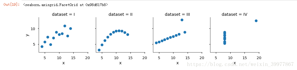
part2:Use Seaborn, visualize all four datasets.
Note:额,做到这里才发现有4个数据集......分4个数据集计算各自的数据特征(part 1)用的方法类似,就不倒回去做part1了......
g = sns.FacetGrid(anascombe, col="dataset")
g.map(plt.scatter, "x","y")
结果:

瓜分20万奖金 获得内推名额 丰厚实物奖励 易参与易上手
更多推荐

 0
0 0
0- 0


 已为社区贡献1条内容

所有评论(0)