手把手教学基于简单神经网络的激光雷达点云车辆检测(附代码)

准备工作pythonmatlabKITTI数据集激光雷达部分参考文献（本文基本按照该文献方式处理）：邓淇天. 基于激光雷达和视觉传感器融合的障碍物识别技术研究[D]. 南京: 东南大学, 2019.1. KITTI数据读入我在https://blog.csdn.net/weixin_43145941/article/details/119513491一文中已经给出了matlab代码用于得到KITT

Y. F. Zhang

5708人浏览 · 2021-08-12 23:26:11

Y. F. Zhang · 2021-08-12 23:26:11 发布

准备工作

python
matlab
KITTI数据集激光雷达部分
参考文献（本文基本按照该文献方式处理）：邓淇天. 基于激光雷达和视觉传感器融合的障碍物识别技术研究[D]. 南京: 东南大学, 2019.
整个项目已push至github（数据部分上传，模型已训练好）：https://github.com/ZYunfeii/KITTI-velodyne-viewer-matlab

1. KITTI数据读入

我在https://blog.csdn.net/weixin_43145941/article/details/119513491一文中已经给出了matlab代码用于得到KITTI点云图。当然，可以假想现在已经获得了一个点云：
$points\_cloud.shape =(n,4)$
其中n为点云个数，4代表点云x,y,z,以及每个点云的反射率。
这一步完成后我们得到如下结果：
在这里插入图片描述
代码（Matlab）：
文件的组织形式参考：https://blog.csdn.net/weixin_43145941/article/details/119513491，否则读文件会读不对位置。

clc; clear; close all;
file = '000019';   % 文件编号 000099 117 19 49

fid=fopen(['./training/velodyne/',file,'.bin'],'rb');
[a,count]=fread(fid,'float32');
fclose(fid);
x = a(1:4:end);
y = a(2:4:end);
z = a(3:4:end);
reflectivity = a(4:4:end);
point_cloud = [x,y,z,reflectivity];
data = pointCloud([x y z]);
figure(1);
pcshow(data);hold on;

label = importdata(['./training/label/',file,'.txt']);
obsName = label.textdata;
data_label = label.data;
obsNum = size(data_label,1); % 包含DontCare类障碍物的总个数
obsCount = 0; % 初始化不包含DontCare类障碍物个数为0

data_calib = importdata(['./training/calib/',file,'.txt']);
Tr_velo_to_cam = reshape(data_calib.data(end-1,:),[4,3])';
Tr_velo_to_cam = [Tr_velo_to_cam;0 0 0 1];

pos = {};  % 创建一个cell数组用于存储障碍物坐标
for i = 1:obsNum
    if obsName{i} == "DontCare"
        continue;
    end
    obsCount = obsCount + 1;
    la = data_label(i,:);
    obsPos = la(11:13)';
    [h,w,l] = deal(la(8),la(9),la(10));
    r_y = la(end);
    
    % obsPos_velo = Tr_cam_to_velo*[obsPos;1];
    % obsPos_velo = obsPos_velo(1:3)
    % t1~t8为障碍物坐标系下的坐标（不考虑障碍物旋转，默认长边与x-axis平行）
    t1 = [l/2,0,w/2];
    t2 = [l/2,0,-w/2];
    t3 = [l/2,-h,w/2];
    t4 = [l/2,-h,-w/2];
    t5 = [-l/2,0,w/2];
    t6 = [-l/2,0,-w/2];
    t7 = [-l/2,-h,w/2];
    t8 = [-l/2,-h,-w/2];
    % 考虑障碍物旋转角度r_y，对x,z方向进行更新
    T = [t1;t2;t3;t4;t5;t6;t7;t8];
    R = [cos(r_y),-sin(r_y);sin(r_y),cos(r_y)];
    T(:,[1,3]) = (R*T(:,[1,3])')';
    % 考虑障碍物坐标系与相机坐标系坐标位移
    T(:,1) = T(:,1) + obsPos(1);
    T(:,2) = T(:,2) + obsPos(2);
    T(:,3) = T(:,3) + obsPos(3);
    % 将相机坐标系转化到激光雷达坐标系
    velo_pos = Tr_velo_to_cam\[T';1,1,1,1,1,1,1,1];
    velo_pos = velo_pos(1:3,:);
    % 记录障碍Box坐标
    pos{i} = velo_pos;
    % 绘制12根线构成3D-Box
    temp = [velo_pos(:,3),velo_pos(:,4),velo_pos(:,7),velo_pos(:,8)];
    [~,j] = max([velo_pos(1,3),velo_pos(1,4),velo_pos(1,7),velo_pos(1,8)]);
    textPoint = temp(:,j);
    text(textPoint(1),textPoint(2),textPoint(3)+0.5,obsName{i},'Color','white');
    plot3(velo_pos(1,[1,2,6,5,1]),velo_pos(2,[1,2,6,5,1]),velo_pos(3,[1,2,6,5,1]),'Color','r');
    plot3(velo_pos(1,[3,4,8,7,3]),velo_pos(2,[3,4,8,7,3]),velo_pos(3,[3,4,8,7,3]),'Color','r');
    plot3(velo_pos(1,[1,3]),velo_pos(2,[1,3]),velo_pos(3,[1,3]),'Color','r');
    plot3(velo_pos(1,[2,4]),velo_pos(2,[2,4]),velo_pos(3,[2,4]),'Color','r');
    plot3(velo_pos(1,[6,8]),velo_pos(2,[6,8]),velo_pos(3,[2,4]),'Color','r');
    plot3(velo_pos(1,[5,7]),velo_pos(2,[5,7]),velo_pos(3,[5,7]),'Color','r');
end

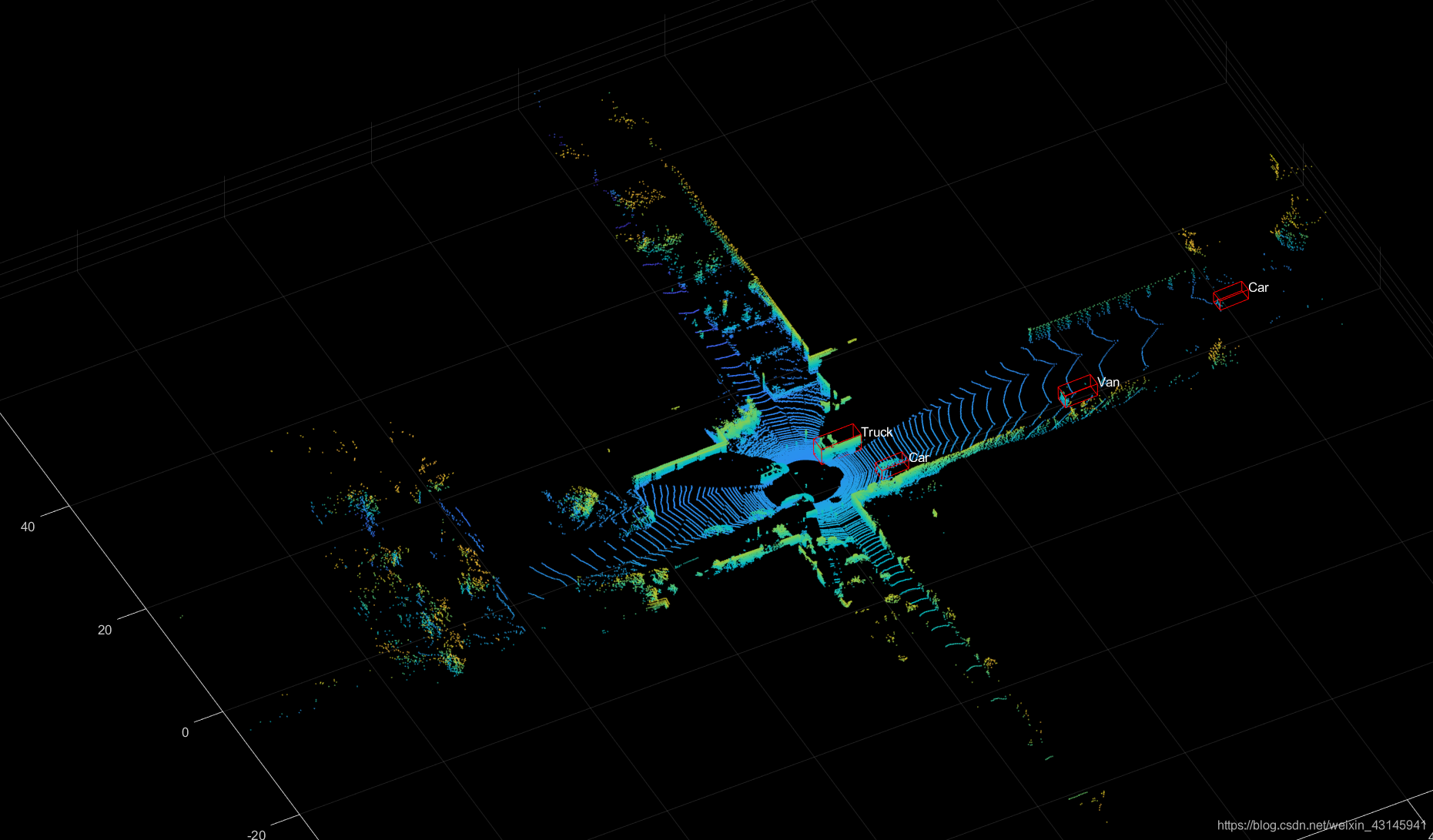
2.障碍物点云提取

在第一步中已经获取到了标注好的3D-Box，也就是知道了Box的地面4个点坐标[(x1,y1,z),(x2,y2,z),(x3,y3,z),(x4,y4,z)]，为了方便提取，将如下区域内的点云视为障碍物点云：
$\{(x,y)|x\in[x_{min},x_{max}],y\in[y_{min},y_{max}]\}\\ x_{min}=min(x_1,x_2,x_3,x_4)\\y_{min}=min(y_1,y_2,y_3,y_4)$
这一部分完成效果如下：
在这里插入图片描述
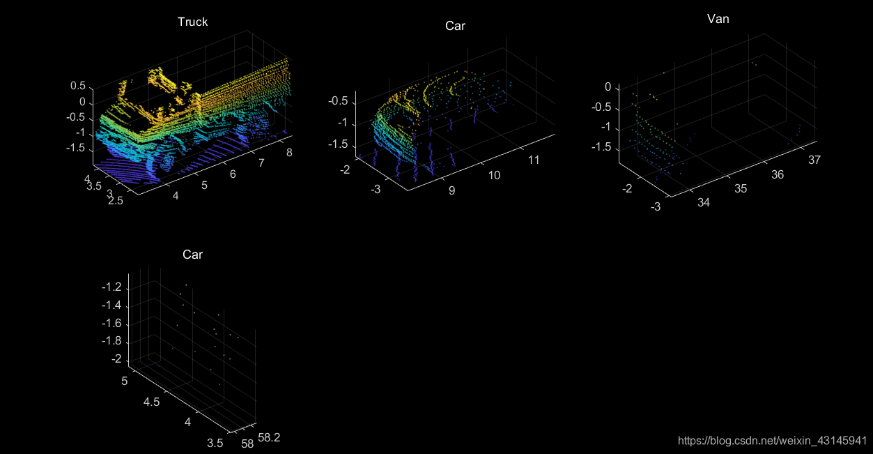
其中有些障碍由于距离激光雷达较远点云较少不具备表征障碍的能力，如上图最后一个。
代码（Matlab）：
接着之前的代码运行。

figure(2);
row = ceil(obsCount / 3);
[n,~] = size(point_cloud);
for k = 1:obsCount
    [max_x,~] = max(pos{k}(1,[1,2,5,6]));   
    [min_x,~] = min(pos{k}(1,[1,2,5,6])); 
    [max_y,~] = max(pos{k}(2,[1,2,5,6]));   
    [min_y,~] = min(pos{k}(2,[1,2,5,6]));
    point_selected = [];
    for i = 1:n
        if point_cloud(i,1)>min_x && point_cloud(i,1)<max_x...
           && point_cloud(i,2)>min_y && point_cloud(i,2)<max_y
            point_selected = [point_selected;point_cloud(i,:)];
        end
    end
    subplot(row,3,k);
    data = pointCloud([point_selected(:,1),point_selected(:,2),point_selected(:,3)]);
    pcshow(data);hold on;
    title(obsName{k});
end

3.去除地面点云

这一部分文献中使用RANSAC算法拟合平面去除地面点云，然而博主试了该算法，运算较慢且易爆内存，不妨采用工程化的思想：激光雷达始终距离车底1.7m左右，而车底与地面基本保持水平，因此可以将点云z坐标小于1.5左右的点视为地面点去除即可。
这一部分完成后效果：
在这里插入图片描述
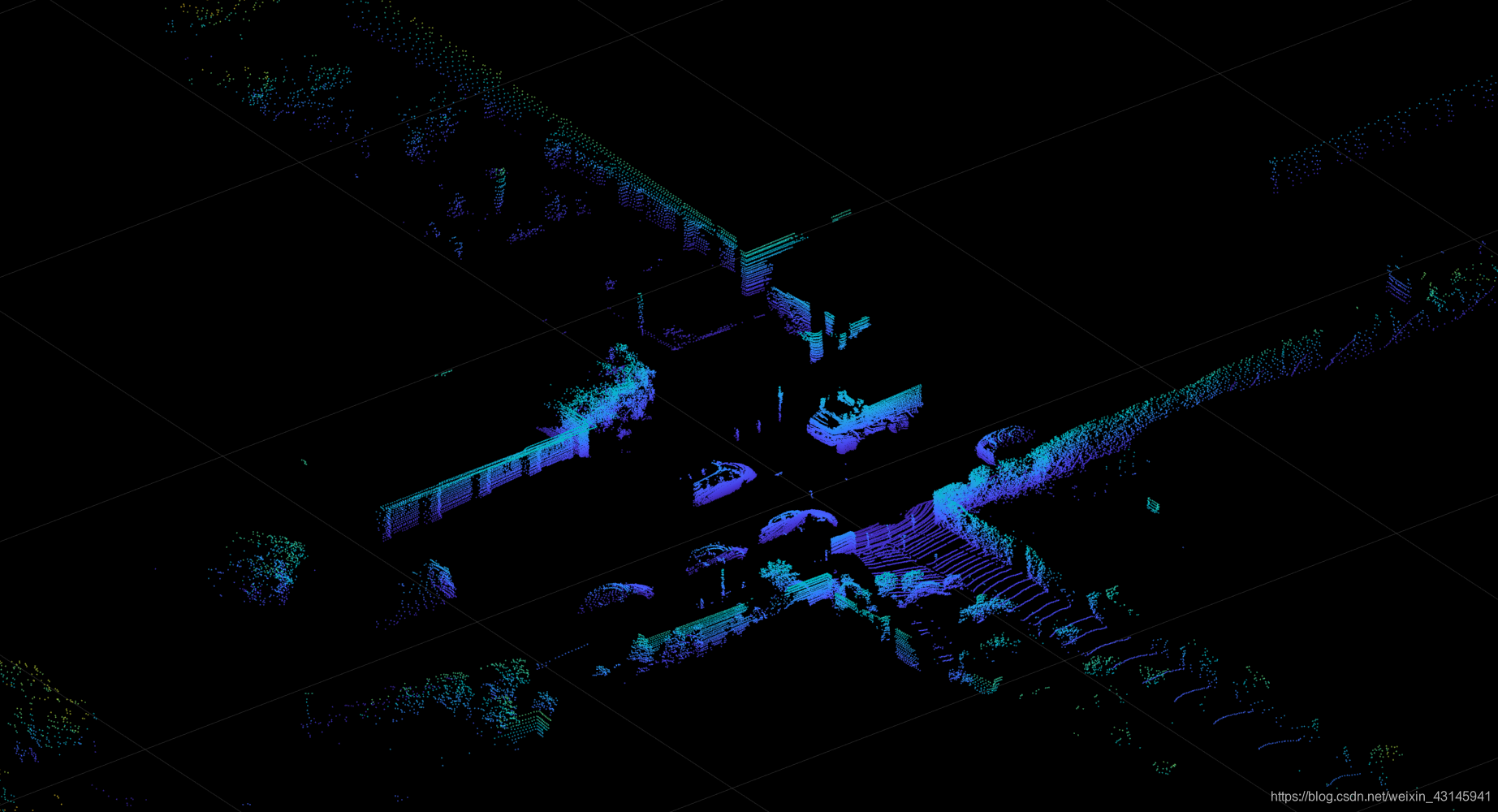
可以明显看到地面点云（水波浪状）被去除。
代码（Matlab）：
接着之前的代码运行。

figure(5);
processed_point_cloud = point_cloud(point_cloud(:,3)>-1.5,:);
data = pointCloud(processed_point_cloud(:,1:3));
pcshow(data);hold on;

4.栅格化点云

为了更好的为后面的处理做准备，一般采用栅格法对点云进行“归类”，即将地图分为一个个的格子，每个格子对应一批次的点云。另外栅格化的好处在于将三维点云二维化，二维只是指其呈现形式，实际上仍旧存储了点云的三维信息以及反射率。在归类后，对每个格子的点云做如下判断：

该格子内的点云高度差是否大于t1；
该格子内的点云数量是否大于t2;
如果1，2均满足，那么保留该格子内的点云，否则舍弃；

这一部分完成后效果：

在这里插入图片描述
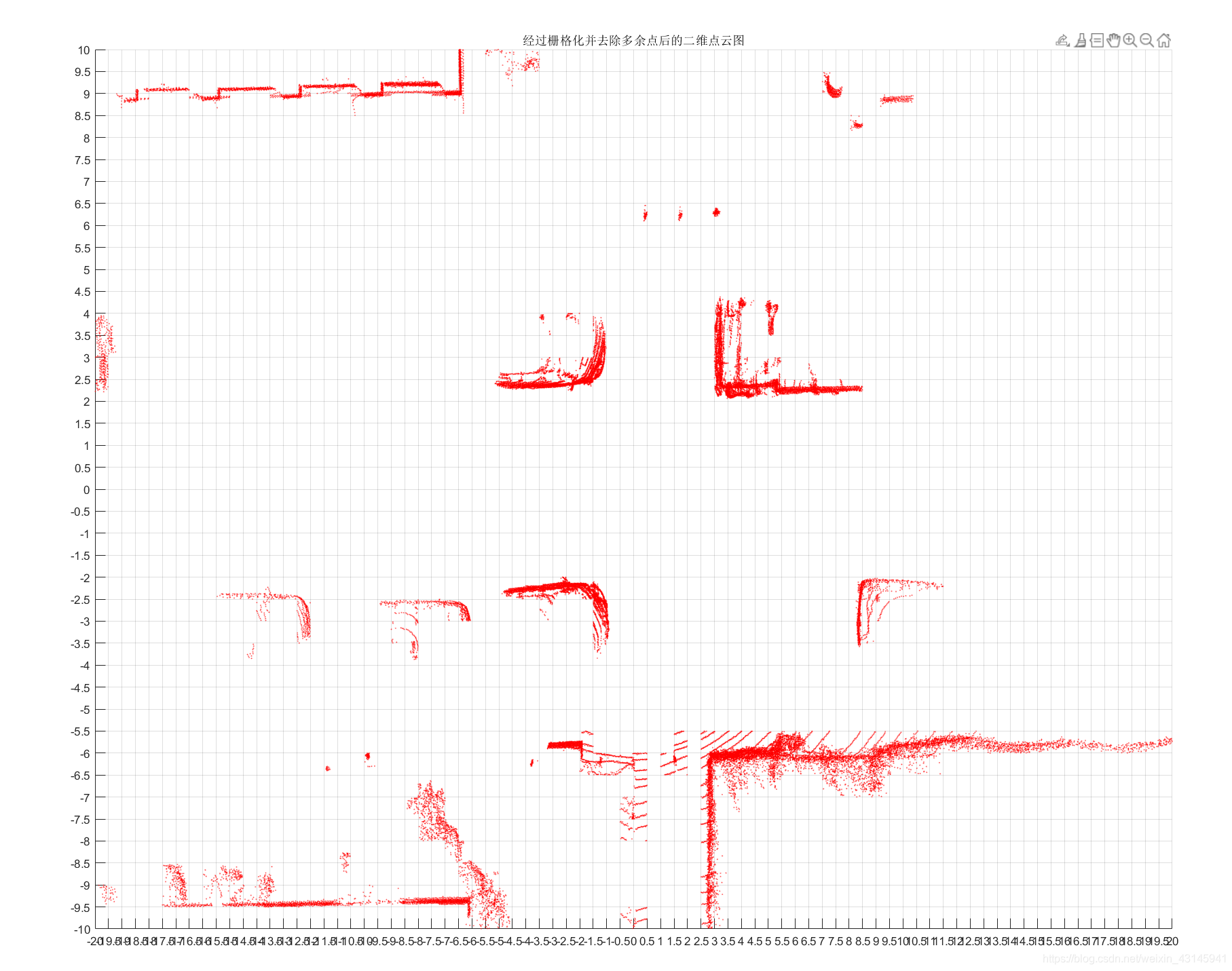
可以看到点云已经有了明显的轮廓，噪音点云也大部分被处理掉。图中心的点云形似"L"，显然它是车辆的点云。
代码（Matlab）：
接着之前的代码运行。

xmin = -20; xmax = 20; ymin = -10; ymax = 10;
d = 0.5;  % 1m*1m栅格尺寸 需要整除xmin and xmax and ymin and ymax
gridcell = cell((xmax-xmin)/d,(ymax-ymin)/d);  % 定义栅格存储cell
for i = 1:size(processed_point_cloud,1)
    point = processed_point_cloud(i,:);
    if point(1)>=xmax || point(1)<=xmin || point(2)>=ymax || point(2)<=ymin
        continue;
    end
    xgrid = ceil((point(1)-xmin)/d);    
    ygrid = ceil((point(2)-ymin)/d); 
    gridcell{xgrid,ygrid} = [gridcell{xgrid,ygrid};point];
end

% 判断有障碍物的栅格将其保留，其余删除
threshold_deltaZ = 0.3;
threshold_point_num = 10;
for i = 1:(xmax-xmin)/d
    for j = 1:(ymax-ymin)/d
        if isempty(gridcell{i,j})
            continue;
        end
        cell_point_count = size(gridcell{i,j},1);
        deltaZ = max(gridcell{i,j}(:,3))-min(gridcell{i,j}(:,3));
        if deltaZ < threshold_deltaZ || cell_point_count < threshold_point_num
            gridcell{i,j} = [];
        end
    end
end

figure(6);
for i = 1:(xmax-xmin)/d
    for j = 1:(ymax-ymin)/d
        if isempty(gridcell{i,j})
            continue;
        end
        scatter(gridcell{i,j}(:,1),gridcell{i,j}(:,2),1,'r.'); hold on;
    end
end
title('经过栅格化并去除多余点后的二维点云图')
set(gca,'XTick',xmin:d:xmax,'YTick',ymin:d:ymax);  % 绘制网格
grid on;

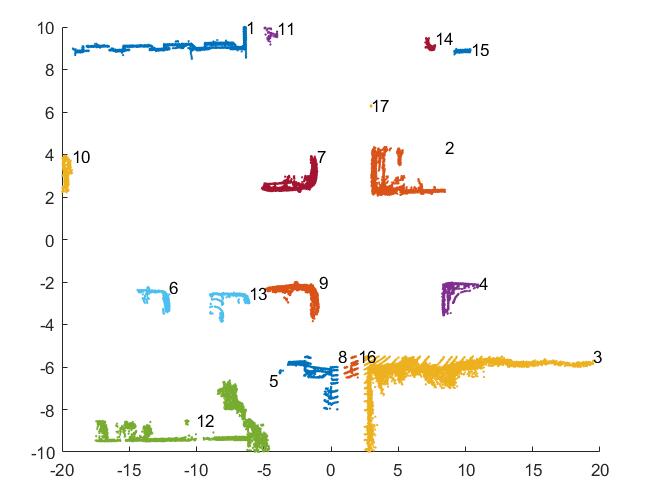
5.DBSCAN栅格聚类

在第4步完成后，我们需要对格子点云进行聚类，由于点云的性质很明显我们需要使用一种基于密度的聚类方法，在机器学习中DBSCAN就是这样一种算法，它的核心思想就是一个元素领域内得有足够的其他元素才能让它属于一类，其聚类效果符合人的直观感受：聚在一起的元素为一类。现成的sklearn中的包或者是其他实现都是直接对点进行DBSCAN聚类，但是我们的点是在栅格内，我们需要对栅格而非直接对点进行聚类，因此需要从零实现。
这一部分实现后效果：
在这里插入图片描述
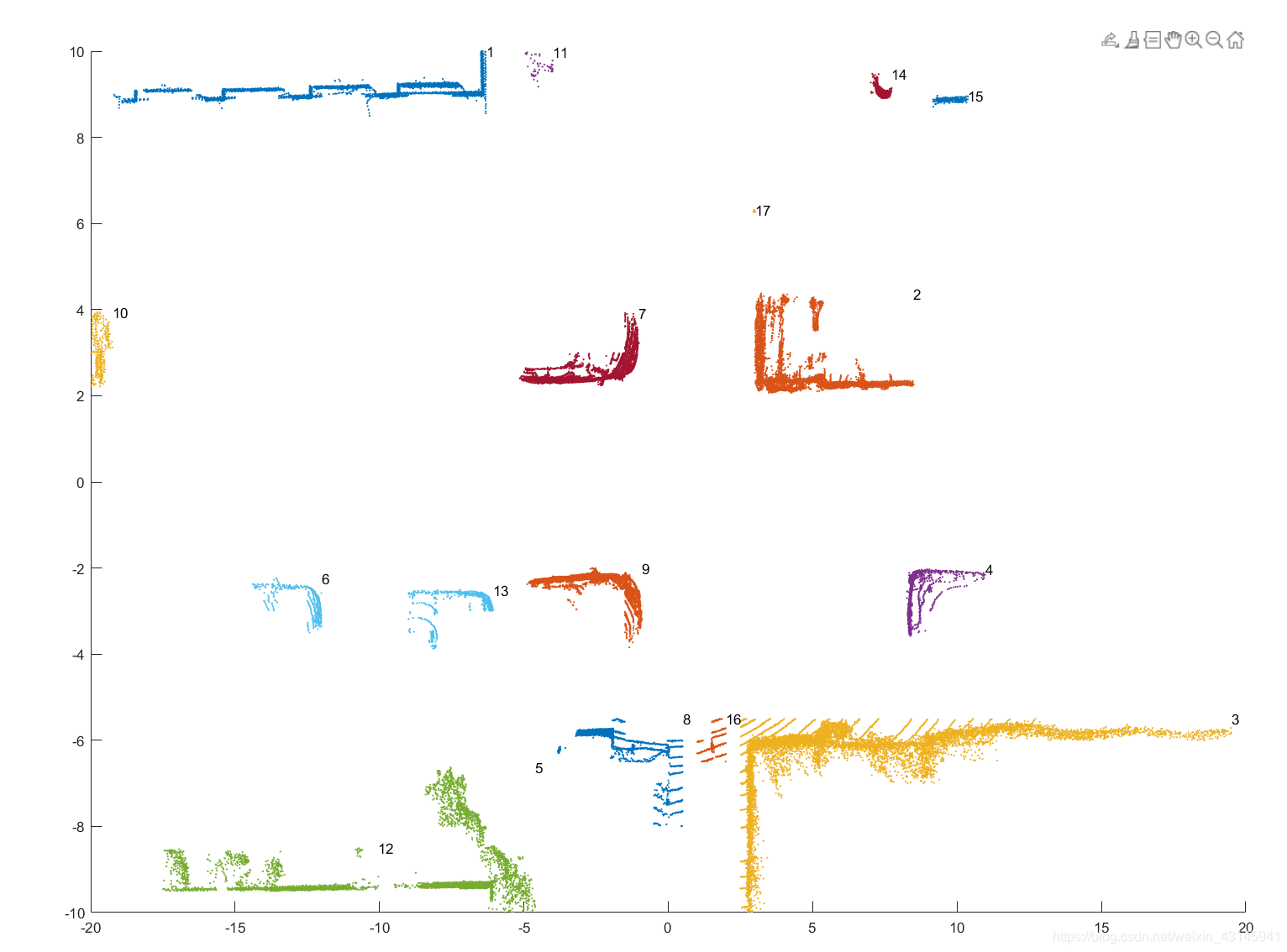
上图为点云聚类后的效果。
代码（Matlab）：
接着之前的代码运行。

cellIndexNotEmpty = [];  % 保存非空的cell的(i,j)
ub = [(xmax-xmin)/d,(ymax-ymin)/d];
lb = [1,1];
for i = 1:ub(1)
    for j = 1:ub(2)
        if isempty(gridcell{i,j})
            continue;
        end
        cellIndexNotEmpty = [cellIndexNotEmpty;i,j 0]; %第三个分量表示栅格是否被访问
    end
end
C = {};  % 聚类类别的cell数组
MinPts = 45; % DBSCAN 参数，领域最小对象数
while any(cellIndexNotEmpty(:,3)==0)
    unvisited_grids = cellIndexNotEmpty(cellIndexNotEmpty(:,3)==0,:);
    random_index = randperm(size(unvisited_grids,1),1);
    p = unvisited_grids(random_index,1:2);
    cellIndexNotEmpty(cellIndexNotEmpty(:,1)==p(1)&cellIndexNotEmpty(:,2)==p(2),3) = 1;  % 标记被访问
    
    neighborhood = [p(1)+1,p(2);p(1)-1,p(2);p(1),p(2)-1;p(1),p(2)+1;...
                    p(1)-1,p(2)-1;p(1)-1,p(2)+1;p(1)+1,p(2)-1;p(1)+1,p(2)+1];
                
    point_num = 0;
    delete_index = [];
    for i = 1:size(neighborhood,1) 
        flag_ub = neighborhood(i,:)>ub;
        flag_lb = neighborhood(i,:)<lb;
        if any(flag_lb+flag_ub)
            delete_index = [delete_index,i];
            continue;
        end
        if isempty(gridcell{neighborhood(i,1),neighborhood(i,2)})
            delete_index = [delete_index,i];
            continue;
        end
        neighbor = neighborhood(i,:);
        point_num = point_num + size(gridcell{neighbor(1),neighbor(2)},1);
    end
    neighborhood(delete_index,:) = [];
    
    if point_num >= MinPts
        if isempty(C)
            C = {p};
        else
            C{end+1} = p;
        end
        while ~isempty(neighborhood)
            neighbor = neighborhood(1,:);
            neighborhood(1,:) = [];
            if cellIndexNotEmpty(cellIndexNotEmpty(:,1)==neighbor(1)&...
               cellIndexNotEmpty(:,2)==neighbor(2),3) == 0
                cellIndexNotEmpty(cellIndexNotEmpty(:,1)==neighbor(1)&...
               cellIndexNotEmpty(:,2)==neighbor(2),3) = 1; % 标记被访问
                neighborhood_ =  [neighbor(1)+1,neighbor(2);neighbor(1)-1,neighbor(2);...
                                 neighbor(1),neighbor(2)-1;neighbor(1),neighbor(2)+1;...
                                 neighbor(1)-1,neighbor(2)-1;neighbor(1)-1,neighbor(2)+1;...
                                 neighbor(1)+1,neighbor(2)-1;neighbor(1)+1,neighbor(2)+1];
                point_num = 0;
                delete_index = [];
                for k = 1:size(neighborhood_,1)
                   flag_ub = neighborhood_(k,:)>ub;
                   flag_lb = neighborhood_(k,:)<lb;
                   if any(flag_lb+flag_ub)
                       delete_index = [delete_index,k];
                       continue;
                   end
                   if isempty(gridcell{neighborhood_(k,1),neighborhood_(k,2)})
                      delete_index = [delete_index,k];
                      continue;
                   end
                   neighbor_ = neighborhood_(k,:);
                   point_num = point_num + size(gridcell{neighbor_(1),neighbor_(2)},1);
                end
                neighborhood_(delete_index,:) = [];
                
                if point_num >= MinPts
                    neighborhood = [neighborhood;neighborhood_];
                    flag = false;
                    for m = 1:size(C,2)
                        temp = C{m};
                        if any(temp(:,1)==neighbor(1)&temp(:,2)==neighbor(2))
                            flag = true;
                            break;
                        end
                    end
                    if ~flag
                        C{end} = [C{end};neighbor];
                    end
                end
            end
        end
    end
end
cluster = {};  % 存放不同类别点云坐标    
figure(7);
for i = 1:size(C,2)
    temp = C{i};
    t2 = [];
    for j = 1:size(temp,1)
        t = temp(j,:);
        x_lb = (t(1)-1)*d+xmin; x_ub = t(1)*d+xmin;
        y_lb = (t(2)-1)*d+ymin; y_ub = t(2)*d+ymin;
        t1 = point_cloud(:,1)>=x_lb & point_cloud(:,1)<=x_ub...
             & point_cloud(:,2)>=y_lb & point_cloud(:,2)<=y_ub...
             & point_cloud(:,3)>-1.5;
        t2 = [t2;point_cloud(t1,:)];
    end
    if isempty(cluster)
        cluster = {t2};
    else
        cluster{end+1} = t2;
    end
    scatter(t2(:,1),t2(:,2),1); hold on;
    text(max(t2(:,1)),max(t2(:,2)),num2str(i))
end
cluster  % 显示本节代码结果（聚类结果）

6.神经网络分类器

点云特征定义

由于聚类后某一类点云数量大且不固定，简单起见，手动计算特征向量。对一类中的点云特征作如下定义（文献简化版）：

点云区域长宽高，3维；
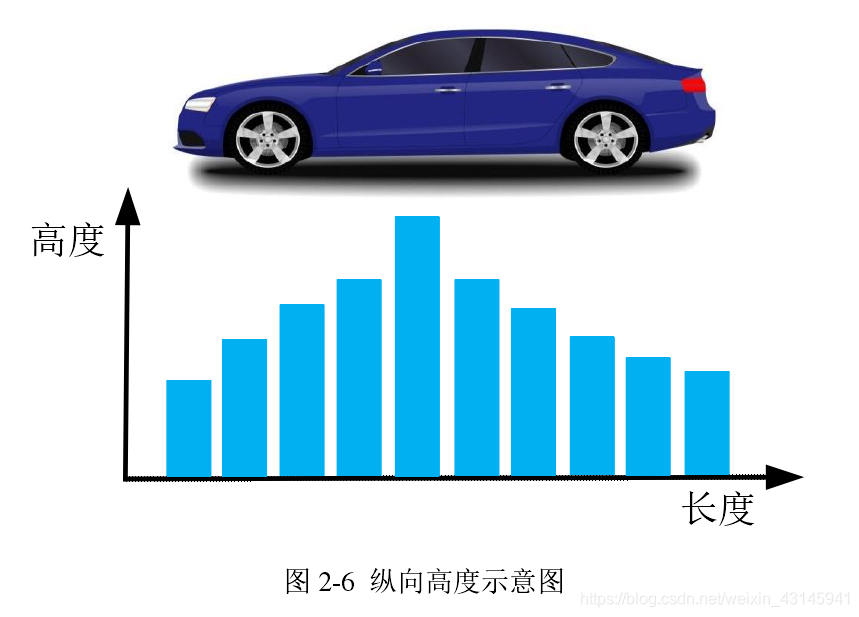
候选目标纵向高度轮廓，取10个区间计算高度z平均值，10维：
点云区域宽高比，1维；
点云平均反射率和方差（汽车反射率高），2维；
反射率占比，1维：
由于存在如下特点：

因此定义特征：
$f=\frac{r e f_{[0,0.2)}-r e f_{[0.2,0.4)}}{P_{n}}$
其中第一个ref表示0到0.2反射率的点云数量，第二个同理可得，Pn为点云总数。

这样对于一个点云簇，可以计算出一个17维特征向量作为分类器输入。

训练集制作

提取KITTI数据集的3D-Box信息和对应障碍物名称，分为car类和others类。

files = dir("./training/velodyne/*.bin");
car_point = {};           % 存储car障碍点云元胞
pedestrian_point = {};     % 存储pedestrain障碍点云元胞
cyclist_point = {};      % 存储cyclist障碍点云元胞
load_file_num = 1000;       % 读取的点云文件数
for k = 1:load_file_num
    filename = files(k).name;
    fid=fopen(['./training/velodyne/',filename],'rb');
    [a,count]=fread(fid,'float32');
    fclose(fid);
    x = a(1:4:end);
    y = a(2:4:end);
    z = a(3:4:end);
    reflectivity = a(4:4:end);  % 反射率
    point_cloud = [x,y,z,reflectivity];
    label = importdata(['./training/label/',filename(1:6),'.txt']);
    data_label = label.data;
    obsName = label.textdata;
    data_calib = importdata(['./training/calib/',filename(1:6),'.txt']);
    Tr_velo_to_cam = reshape(data_calib.data(end-1,:),[4,3])';
    Tr_velo_to_cam = [Tr_velo_to_cam;0 0 0 1];
    pos = {};                 % 创建一个cell数组用于存储障碍物坐标
    obsNum = size(obsName,1); % 包含DontCare类障碍物的总个数
    for i = 1:obsNum
        if obsName{i} == "DontCare"
            continue;
        end
        la = data_label(i,:);
        obsPos = la(11:13)';
        [h,w,l] = deal(la(8),la(9),la(10));
        r_y = la(end);
        % t1~t8为障碍物坐标系下的坐标（不考虑障碍物旋转，默认长边与x-axis平行）
        t1 = [l/2,0,w/2];
        t2 = [l/2,0,-w/2];
        t3 = [l/2,-h,w/2];
        t4 = [l/2,-h,-w/2];
        t5 = [-l/2,0,w/2];
        t6 = [-l/2,0,-w/2];
        t7 = [-l/2,-h,w/2];
        t8 = [-l/2,-h,-w/2];
        % 考虑障碍物旋转角度r_y，对x,z方向进行更新
        T = [t1;t2;t3;t4;t5;t6;t7;t8];
        R = [cos(r_y),-sin(r_y);sin(r_y),cos(r_y)];
        T(:,[1,3]) = (R*T(:,[1,3])')';
        % 考虑障碍物坐标系与相机坐标系坐标位移
        T(:,1) = T(:,1) + obsPos(1);
        T(:,2) = T(:,2) + obsPos(2);
        T(:,3) = T(:,3) + obsPos(3);
        % 将相机坐标系转化到激光雷达坐标系
        velo_pos = Tr_velo_to_cam\[T';1,1,1,1,1,1,1,1];
        velo_pos = velo_pos(1:3,:);
        % 记录障碍Box坐标
        pos{i} = velo_pos;
    end

    [n,~] = size(point_cloud);
    
    for i = 1:obsNum
        if obsName{i} == "DontCare"
            continue;
        end
        [max_x,~] = max(pos{i}(1,[1,2,5,6]));   
        [min_x,~] = min(pos{i}(1,[1,2,5,6])); 
        [max_y,~] = max(pos{i}(2,[1,2,5,6]));   
        [min_y,~] = min(pos{i}(2,[1,2,5,6]));
        la = data_label(i,:);
        [h,w,l] = deal(la(8),la(9),la(10));
        point_selected = [];
        for j = 1:n
            if point_cloud(j,1)>min_x && point_cloud(j,1)<max_x...
               && point_cloud(j,2)>min_y && point_cloud(j,2)<max_y && point_cloud(j,3)>-1.5
                point_selected = [point_selected;point_cloud(j,:)];
            end
        end
        point_selected = [l,w,h,0;point_selected];   % 数据集第一行数据为[l w h 0],0只是占位
        if obsName{i} == "Car" && size(point_selected,1)>200
            if isempty(car_point)
                car_point = {point_selected};
            else
                car_point{end+1} = point_selected;
            end
        end
        if obsName{i} == "Pedestrian" && size(point_selected,1)>100
            if isempty(pedestrian_point)
                pedestrian_point = {point_selected};
            else
                pedestrian_point{end+1} = point_selected;
            end
        end
        if obsName{i} == "Cyclist" && size(point_selected,1)>100
            if isempty(cyclist_point)
                cyclist_point = {point_selected};
            else
                cyclist_point{end+1} = point_selected;
            end
        end
    end
end

figure(8);
pcshow(pointCloud(pedestrian_point{3}(2:end,1:3)))

for i = 1:size(car_point,2)
    writematrix(car_point{i},['./training/car/',num2str(i),'.csv']);   
end
for i = 1:size(pedestrian_point,2)
    writematrix(pedestrian_point{i},['./training/pedestrian/',num2str(i),'.csv']);
end
for i = 1:size(cyclist_point,2)
    writematrix(cyclist_point{i},['./training/cyclist/',num2str(i),'.csv']);
end

将聚类点云簇保存为csv

聚类的结果是用于之后Python模型的，因此保存一下结果。

% cluster点云存储
for i = 1:size(cluster,2)
    temp = cluster{i};
    max_x = max(temp(:,1));
    min_x = min(temp(:,1));
    max_y = max(temp(:,2));
    min_y = min(temp(:,2));
    h = max(temp(:,3)) - min(temp(:,3));
    if max_x - min_x > max_y - min_y
        l = max_x - min_x;
        w = max_y - min_y;
    else
        l = max_y - min_y;
        w = max_x - min_x;
    end
    writematrix([l,w,h,0;temp],['./testing/cluster/',num2str(i),'.csv']); 
end

在这里插入图片描述
每个csv表示一帧点云图中一个点云簇的点云矩阵，这个点云矩阵还附加了一行用以携带这个点云簇的长宽高，用以特征向量计算。

特征向量Python计算

从现在开始均为Python程序。
按照之前特征向量的计算方式编写即可：

#!/usr/bin/python
# -*- coding: UTF-8 -*-

"""
Date: 2021.8.11
Author: Y. F. Zhang
"""

from sklearn.model_selection import train_test_split
import matplotlib.pyplot as plt
import torch
from torch import nn
import pandas as pd
import numpy as np
import os

feature_dim = 15
device = 'cuda' if torch.cuda.is_available() else 'cpu'

def feature_extract(filename):
    data = pd.read_csv(filename,header=None).to_numpy(dtype=float)
    point_cloud = data[1:,0:3]
    ref = data[1:,3]
    [l,w,h,_] = data[0,:]
    max_x,min_x = np.max(point_cloud[:,0]),np.min(point_cloud[:,0])
    max_y, min_y = np.max(point_cloud[:,1]), np.min(point_cloud[:,1])
    # f1 = np.array([l,w,h])                          # 第一个特征
    f1 = np.array([h])   # 仅用h效果好些

    slices_num = 10
    if max_x-min_x > max_y-min_y:
        t = np.linspace(min_x,max_x,slices_num+1)   # slices_num+1个值构成slices_num个区间
        flag = 0
    else:
        t = np.linspace(min_y, max_y, slices_num+1)
        flag = 1
    f2 = []
    for i in range(len(t)-1):
        lb,ub = t[i],t[i+1]
        sum_h,num = 0,0
        for point in point_cloud:
            if lb < point[flag] < ub:
                sum_h += point[2]
                num += 1
        f2.append(sum_h/num if num!=0 else 0)
    f2 = np.array(f2)                                            # 第二个特征
    f3 = np.array([(max_x-min_x if flag==1 else max_y-min_y)/h]) # 第三个特征
    f4 = np.array([np.mean(ref),np.std(ref)])                    # 第四个特征
    num1,num2 = 0,0
    for r in ref:
        if 0<=r<0.2:
            num1 += 1
        if 0.2<=r<0.4:
            num2 += 1
    f5 = np.array([(num1 - num2) / point_cloud.shape[0]])  # 第五个特征
    feature = np.concatenate((f1,f2,f3,f4,f5))
    return feature

加载数据以及DataLoader制作

这一部分比较基础，直接看代码就能懂，唯一想解释一下的是我将行人和自行车都视为了“非car类”，并标记为1，“car”标记为0：

def load_data():
    data_car = np.array([[]],dtype=float).reshape(-1,feature_dim)
    for file in os.listdir('./training/car'):
        data_car = np.concatenate((data_car,feature_extract('./training/car/'+file).reshape(1,-1)),axis=0)
    label_car = np.zeros((data_car.shape[0],),dtype=float)   # car标记为0

    data_pedestrian = np.array([[]], dtype=float).reshape(-1, feature_dim)
    for file in os.listdir('./training/pedestrian'):
        data_pedestrian = np.concatenate((data_pedestrian, feature_extract('./training/pedestrian/' + file).reshape(1, -1)), axis=0)
    label_pederstian = 1+np.zeros((data_pedestrian.shape[0],), dtype=float)   # pedestrian标记为1

    data_cyclist = np.array([[]], dtype=float).reshape(-1, feature_dim)
    for file in os.listdir('./training/cyclist'):
        data_cyclist = np.concatenate((data_cyclist, feature_extract('./training/cyclist/' + file).reshape(1, -1)),axis=0)
    label_cyclist = 1+np.zeros((data_cyclist.shape[0],), dtype=float)  # cyclist标记为1

    data_others = np.array([[]], dtype=float).reshape(-1, feature_dim)
    for file in os.listdir('./training/others'):
        data_others = np.concatenate((data_others, feature_extract('./training/others/' + file).reshape(1, -1)),axis=0)
    label_others = 1 + np.zeros((data_others.shape[0],), dtype=float)  # others标记为1

    total_data = np.concatenate((data_car,data_pedestrian,data_cyclist,data_others),axis=0)
    total_label = np.concatenate((label_car,label_pederstian,label_cyclist,label_others))

    train_x,test_x,train_y,test_y = train_test_split(total_data,total_label)


    train_x = torch.from_numpy(train_x).type(torch.float32).to(device)
    train_y = torch.from_numpy(train_y).type(torch.LongTensor).to(device)
    test_x = torch.from_numpy(test_x).type(torch.float32).to(device)
    test_y = torch.from_numpy(test_y).type(torch.LongTensor).to(device)

    class Mydataset(torch.utils.data.Dataset):
        def __init__(self, features, labels):
            self.features = features
            self.labels = labels

        def __getitem__(self, index):
            feature = self.features[index]
            label = self.labels[index]
            return feature, label

        def __len__(self):
            return len(self.features)

    train_ds = Mydataset(train_x, train_y)
    test_ds = Mydataset(test_x, test_y)
    BTACH_SIZE = 256
    train_dl = torch.utils.data.DataLoader(
                train_ds,
                batch_size=BTACH_SIZE,
                shuffle=True)
    test_dl = torch.utils.data.DataLoader(
                test_ds,
                batch_size=BTACH_SIZE,
                shuffle=True)
    print('=====load data finished!+=====')
    return train_dl,test_dl,(train_ds,test_ds)

模型搭建

这一部分是最简单的，因为这个分类问题其实并不复杂，特征都是手动提取的，网络只需要简单拟合一下，因此就用MLP即可，输入维度17，对应特征维度，输出维度2，对应是car和others的概率。这里我使用交叉熵函数CrossEntropyLoss，注意这个函数内部其实会实现一个softmax，因此网络输出线性层即可。这里其实用sigmod一维输出也是可以的，损失函数用BCELoss。

def get_model():
    class Model(nn.Module):
        def __init__(self,dim):
            super().__init__()
            self.liner_1 = nn.Linear(dim,256)
            self.liner_2 = nn.Linear(256,256)
            self.liner_3 = nn.Linear(256,2)
            self.relu = nn.LeakyReLU()
        def forward(self,feature):
            x = self.liner_1(feature)
            x = self.relu(x)
            x = self.liner_2(x)
            x = self.relu(x)
            x = self.liner_3(x)
            return x

    model = Model(feature_dim).to(device)
    opt = torch.optim.Adam(model.parameters(),lr=1e-4)
    loss_fn = nn.CrossEntropyLoss()
    return model,opt,loss_fn

训练模型

到这一步代码基本就是复制粘贴：

def main():
    train_dl,test_dl,(train_ds,test_ds) = load_data()
    model,opt,loss_fn = get_model()

    def accuracy(y_pred,y_true):
        y_pred = torch.argmax(y_pred,dim=1)
        acc = (y_pred == y_true).float().mean()
        return acc

    epochs = 400
    loss_list = []
    accuracy_list = []
    test_loss_list = []
    test_accuarcy_list = []
    for epoch in range(epochs):
        model.train()
        for x, y in train_dl:
            if torch.cuda.is_available():
                x, y = x.to('cuda'), y.to('cuda')
            y_pred = model(x)
            loss = loss_fn(y_pred, y)
            opt.zero_grad()
            loss.backward()
            opt.step()

        model.eval()
        with torch.no_grad():
            epoch_accuracy = accuracy(model(train_ds.features), train_ds.labels)
            epoch_loss = loss_fn(model(train_ds.features), train_ds.labels).data
            epoch_test_accuracy = accuracy(model(test_ds.features), test_ds.labels)
            epoch_test_loss = loss_fn(model(test_ds.features), test_ds.labels).data
            loss_list.append(round(epoch_loss.item(), 3))
            accuracy_list.append(round(epoch_accuracy.item(), 3))
            test_loss_list.append(round(epoch_test_loss.item(), 3))
            test_accuarcy_list.append(round(epoch_test_accuracy.item(), 3))
            print('epoch: ', epoch, 'loss： ', round(epoch_loss.item(), 3),
                  'accuracy:', round(epoch_accuracy.item(), 3),
                  'test_loss： ', round(epoch_test_loss.item(), 3),
                  'test_accuracy:', round(epoch_test_accuracy.item(), 3)
                  )
    save_model_para(model)
    torch.save(model.state_dict(),'model_state_dict.pkl')
    plt.figure(1)
    plt.plot(range(0, epochs), loss_list, 'r', label='Training loss')
    plt.plot(range(0, epochs), accuracy_list, 'g', label='Training accuracy')
    plt.plot(range(0, epochs), test_loss_list, 'b', label='Test loss')
    plt.plot(range(0, epochs), test_accuarcy_list, 'k', label='Test accuracy')
    plt.title('Training and Validation Loss')
    plt.xlabel('Epoch')
    plt.legend()
    plt.show()

if __name__ == "__main__":
    def setup_seed(seed):
        """设置随机数种子函数"""
        torch.manual_seed(seed)
        torch.cuda.manual_seed_all(seed)
        np.random.seed(seed)
        torch.backends.cudnn.deterministic = True
    setup_seed(188)
    test()

learning curve：
在这里插入图片描述
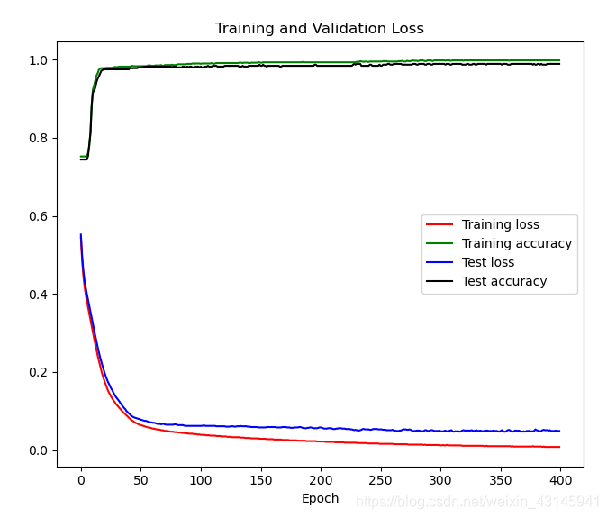
由于任务简单，一下就训练好了…

测试函数

用之前聚类结果来测试一下：

def test():
    model = get_model()[0]
    model.load_state_dict(torch.load('model_state_dict.pkl'))
    test_feature = np.array([[]], dtype=float).reshape(-1, feature_dim)
    test_data = list()
    for file in os.listdir('./testing/cluster'):
        data = pd.read_csv("".join(['./testing/cluster/',file]), header=None).to_numpy(dtype=float)
        test_data.append(data)
        feature = feature_extract("".join(['./testing/cluster/',file]))
        test_feature = np.concatenate((test_feature,feature.reshape(1,-1)),axis=0)
    test_x = torch.from_numpy(test_feature).type(torch.float32).to(device)

    model.eval()
    plt.figure(2)
    plt.scatter(0,0,s=20)
    with torch.no_grad():
        output = model(test_x)
        y_pred = torch.argmax(output,dim=1).cpu().detach().numpy()
        points_dict = {'Car':np.array([]),'Others':np.array([])}
        category_list = ['Car','Others']
        for i,val in enumerate(y_pred):
            points_dict[category_list[val]] = np.append(points_dict[category_list[val]],test_data[i][1:,0:3])
        for ca in category_list:
            points = points_dict[ca].reshape(-1,3)
            plt.scatter(points[:,0],points[:,1],s=np.ones(len(points),))
        leg = ['Coordinate origin of lidar']
        leg.extend(category_list)
        plt.legend(leg)
    plt.show()

在这里插入图片描述
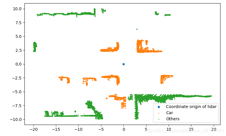
基本实现功能。这里可能还是会出现某些识别错误，这也是激光雷达的弊端。由于在点云处理的时候可能把原本属于一个障碍物的某部分稀疏点云去除了，导致识别有误。另外当障碍物距离激光雷达较远时点云较少，特征很难被识别也会出错，只有当障碍物靠近激光雷达时本文的模型才能较好地识别出它是否为Car。

最终结果

由于训练集中针对3D-Box的标注很大程度上存在人为的先验知识即虽然某个区域点云稀疏但标注的人知道实际上该区域仍旧属于障碍物并把它标入Box，而最终测试阶段使用的是聚类后的点云，稀疏区域的点云被过滤掉了，这样导致类簇的长宽都可能大幅度减小（尤其是距离激光雷达远的时候，远离激光雷达的一端点云少甚至没有），为了在测试阶段依旧让网路明白类簇是否为Car，因此决定将原本第一个特征定义即长宽高改为只使用高，特征向量维度从17变为15。下面是某一帧结果：
在这里插入图片描述
全部分类正确。