感谢大家的收藏，我会继续完善这篇博客的 😄 ❤️

定义

泰勒图：泰勒图¹常用于评价模型的精度，常用的精度指标有相关系数，标准差以及均方根误差(RMSE)。一般而言，泰勒图中的散点代表模型，辐射线代表相关系数，横纵轴代表标准差，而虚线代表均方根误差。泰勒图一改以往用散点图这种只能呈现两个指标来表示模型精度的情况。从更广义地来讲，泰勒图可以延展到需要用二维平面呈现三维数据的应用场景。这一点与三元图有异曲同工之妙。

功能：相关/分布描述

Taylor skill score (TSS) 是泰勒图的数值总结，可以反映预测技能的综合指标，其中0表示least skill，1表示most skill。综合测定相关系数、标准差，RMSE。
对于任何给定的方差，TSS随相关性(r接近r0)的增加而单调增加;对于任何给定的相关性，随着建模方差接近观测方差(标准差比或SDR 1)而增加。

$TSS=\frac{4(1+r{)}^4}{(SDR+\frac{1}{SDR}{)}^2(1+r_0{)}^4}$

$r=\frac{\frac{1}{n}{\sum }_{i=1}^n(X_i-\overline{X})(Y_i-\overline{Y})}{{\sigma }_X{\sigma }_Y}$

$SDR=\frac{{\sigma }_X}{{\sigma }_Y}$

${\sigma }_X=\sqrt{\frac{{\sum }_{i=1}^n(X_i-\overline{X}{)}^2}{n}}$，${\sigma }_Y=\sqrt{\frac{{\sum }_{i=1}^n(Y_i-\overline{Y}{)}^2}{n}}$，
$r_0$是可获得的最大相关性，通常设置为0.999。

例子

案例1

案例2²

这里只描述了两种指标，归一化标准差和相关系数

拓展

还有一种综合指标的反映KGE(Kling–Gupta efficiency) 测量观测值与模拟值之间一致性的综合准则范围为-∞ ~ 1，最优值为1

$KGE=1-\sqrt{(r-1{)}^2+(\beta -1{)}^2+(\gamma -1{)}^2}$

这里$r$为Pearson相关系数，$\beta$为偏倚项(即均值之比)，$\gamma$为变异性项(即变异系数之比，观测数据的标准差之比)。

英文原版定义

A Taylor diagram provides a statistical summary of how well patterns match and is widely used to compare the outputs from models with observations1. Supplementary Figure 1 shows a comparison of the globally averaged seasonal time series (climatology for 1980 2005) from models and the GRACE observations (climatology for 2003 2012). First, the correlation coefficients for the radial line denote the relationship between GRACE and the models, indicating similarities on seasonal time scales. Second, the normalized standard deviations (standard deviation of the model divided by that of the observations) on the x- and y-axes indicate if the variance of the model is larger or smaller than those in the observations. The points inside the dashed curved line mean that the model simulations have lower variability than the GRACE observations. By contrast, the models with normalized standard deviation are higher than one has higher variability than the GRACE observations. For example, GISS observations have more than two times the standard deviation of the GRACE observations because of a larger seasonal cycle. The reasons for the biases in the model could be from simulated atmospheric forcing from the configurations, such as soil type, layers, and depths, or parameterizations in different land surface models. On combining the correlation and standard deviation, the points closer to the reference point on the x-axis show a better agreement, making the ensemble mean of the CESM-LE one of the realistic models representing terrestrial water storage. Supplementary Figure 1 shows that the CESM agrees with observations for the simulated seasonal cycle of total water storage.

python绘图方法

超干货 | 泰勒图(Taylor diagram)绘制方法大汇总

一个例子

import matplotlib.pyplot as plt
from matplotlib import rcParams
import numpy as np
import pandas  as pd
import skill_metrics as sm
 
data = pd.read_excel(r"test_data.xlsx")
# 以下操作可以当作固定步骤
taylor_stats1 = sm.taylor_statistics(data.pred1,data.ref,'data')
taylor_stats2 = sm.taylor_statistics(data.pred2,data.ref,'data')
taylor_stats3 = sm.taylor_statistics(data.pred3,data.ref,'data')
sdev = np.array([taylor_stats1['sdev'][0], taylor_stats1['sdev'][1], 
                 taylor_stats2['sdev'][1], taylor_stats3['sdev'][1]])
crmsd = np.array([taylor_stats1['crmsd'][0], taylor_stats1['crmsd'][1], 
                  taylor_stats2['crmsd'][1], taylor_stats3['crmsd'][1]])
ccoef = np.array([taylor_stats1['ccoef'][0], taylor_stats1['ccoef'][1], 
                  taylor_stats2['ccoef'][1], taylor_stats3['ccoef'][1]])
 
# 设置matplotlib 基本配置
rcParams["figure.figsize"] = [6, 6]
rcParams["figure.facecolor"] = "white"
rcParams["figure.edgecolor"] = "white"
rcParams["figure.dpi"] = 80
rcParams['lines.linewidth'] = 1 # 
rcParams["font.family"] = "Times New Roman"
rcParams.update({'font.size': 12}) # 
plt.close('all')
# 开始绘图
text_font = {'size':'15','weight':'bold','color':'black'}
sm.taylor_diagram(sdev,crmsd,ccoef)
plt.title("Example01 Of taylor_diagram() in Python",fontdict=text_font,pad=35)

数据格式excel，列名分别为pred1，pred2，pred3，ref
每一个列名pred1是一个序列值，ref是一个序列值，一个数据有一个pred和一个ref成对计算，最终在图上有多少下，就有多少个pred，对应这里是pred_n, taylor_stats1[‘sdev’][0]是列名

参考skill_metric

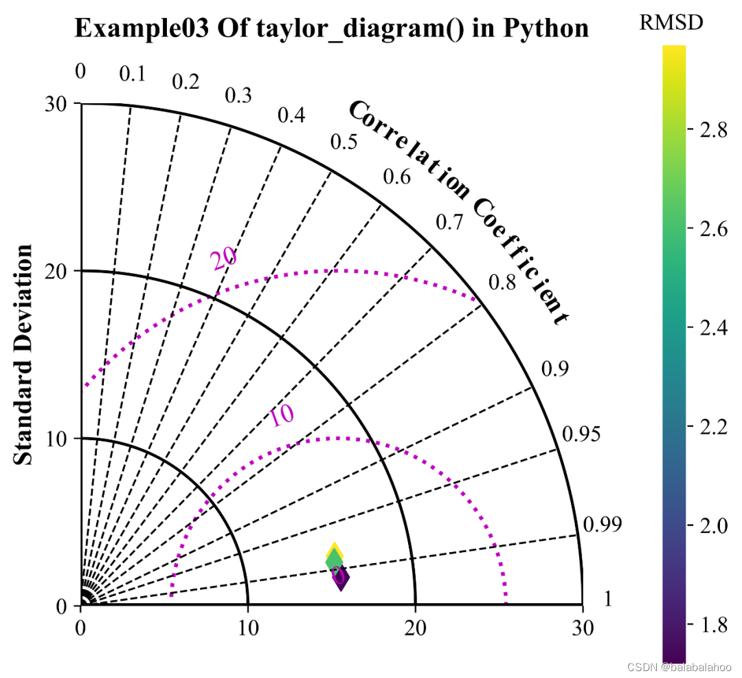
sm.taylor_diagram(sdev,crmsd,ccoef,
                      markerDisplayed = 'colorBar', titleColorbar = 'RMSD',
                     locationColorBar = 'EastOutside',
                      cmapzdata = crmsd, titleRMS = 'off',
                      tickRMS = range(0,30,10), tickRMSangle = 110.0,
                      colRMS = 'm', styleRMS = ':', widthRMS = 2.0,
                      tickSTD = range(10,30,10), axismax = 30.0,
                      colSTD = 'k', styleSTD = '-', widthSTD = 1.5,
                      colCOR = 'k', styleCOR = '--', widthCOR = 1.0)
text_font = {'size':'15','weight':'bold','color':'black'}
plt.title("Example03 Of taylor_diagram() in Python",fontdict=text_font,pad=35)

---

1. Taylor K E. Summarizing multiple aspects of model performance in a single diagram[J]. Journal of Geophysical Research: Atmospheres, 2001, 106(D7): 7183-7192. ↩︎

2. WU W Y, LO M H, WADA Y等, 2020. SI-Divergent effects of climate change on future groundwater availability in key mid-latitude aquifers[J/OL]. Nature Communications, 11(1). DOI:10.1038/s41467-020-17581-y. ↩︎