
深度学习基础(四) -- pandas基础知识
pandas 是基于NumPy 的一种工具,该工具是为了解决数据分析任务而创建的。Pandas 纳入了大量库和一些标准的数据模型,提供了高效地操作大型数据集所需的工具。pandas提供了大量能使我们快速便捷地处理数据的函数和方法。1、DataFrame结构pandas 相当于 python 中 excel:它使用表(也就是 dataframe),能在数据上做各种变换,但还有其他很多功能。D...
pandas 是基于NumPy 的一种工具,该工具是为了解决数据分析任务而创建的。Pandas 纳入了大量库和一些标准的数据模型,提供了高效地操作大型数据集所需的工具。pandas提供了大量能使我们快速便捷地处理数据的函数和方法。
在pandas中主要有两种数据类型,可以简单的理解为:
- Series:一维数组
- DateFrame:二维数组(矩阵)
引入对应的包:
import numpy as np
import pandas as pd
新建对象 Object Creation
- series
可以通过传入一个list对象来新建Series,其中空值为np.nan:
s = pd.Series([1,3,4,np.nan,7,9])
s

out[5]:
0    1.0
1    3.0
2    4.0
3    NaN
4    7.0
5    9.0
dtype: float64
x x x
pandas会默认创建一列索引index(上面的0-5)。我们也可以在创建时就指定索引:
pd.Series([1,3,4,np.nan,7,9], index=[1,1,2,2,'a',4])

Out[6]:
1    1.0
1    3.0
2    4.0
2    NaN
a    7.0
4    9.0
dtype: float64
注意的是,索引是可以重复的,也可以是字符。
- DataFrame
新建一个DataFrame对象可以有多种方式:
通过传入一个numpy的数组、指定一个时间的索引以及一个列名。
dates = pd.date_range('20190101', periods=6)
dates
Out[11]:
DatetimeIndex(['2019-01-01', '2019-01-02', '2019-01-03', '2019-01-04',
               '2019-01-05', '2019-01-06'],
              dtype='datetime64[ns]', freq='D')
df = pd.DataFrame(np.random.randn(6,4), index=dates, columns=list('ABCD'))
df
Out[18]:
                   A         B         C         D
2019-01-01  0.671622  0.785726  0.392435  0.874692
2019-01-02 -2.420703 -1.116208 -0.346070  0.785941
2019-01-03  1.364425 -0.947641  2.386880  0.585372
2019-01-04 -0.485980 -1.281454  0.354063 -1.418858
2019-01-05 -1.122717 -2.789041 -0.791812 -0.174345
2019-01-06  0.221597 -0.753038 -1.741256  0.287280
通过传入一个dict对象
df2 = pd.DataFrame({'A':1.,
                    'B':pd.Timestamp('20190101'),
                    'C':pd.Series(1, index=list(range(4)), dtype='float32'),
                    'D':np.array([3]*4, dtype='int32'),
                    'E':pd.Categorical(["test", "tain", "test", "train"]),
                    'F':'foo'})
df2
Out[27]:
     A          B    C  D      E    F
0  1.0 2019-01-01  1.0  3   test  foo
1  1.0 2019-01-01  1.0  3   tain  foo
2  1.0 2019-01-01  1.0  3   test  foo
3  1.0 2019-01-01  1.0  3  train  foo
们指定了不同的类型,可以通过如下查看:
df2.dtypes
Out[28]:
A           float64
B    datetime64[ns]
C           float32
D             int32
E          category
F            object
dtype: object
可以看出DataFrame和Series一样,在没有指定索引时,会自动生成一个数字的索引,这在后续的操作中十分重要。
查看 Viewing Data
- 查看开头几行或者末尾几行:
使用head可以查看前几行的数据,默认的是前5行,不过也可以自己设置。
使用tail可以查看后几行的数据,默认也是5行,参数可以自己设置
并且可以通过添加行数参数来输出
df.head()  # 只看前3行:df4.head(3)
Out[13]:
                   A         B         C         D
2019-01-01 -2.461184  1.201754 -0.268156 -0.668064
2019-01-02  0.125445  0.809079 -0.249266 -1.822513
2019-01-03  0.251630  0.943034  0.549889  0.254871
2019-01-04 -1.976977 -0.411209  1.886561 -0.018010
2019-01-05  0.534982 -1.600566  0.153771  0.361376

df.tail(3)
Out[14]:
                   A         B         C         D
2019-01-04 -1.976977 -0.411209  1.886561 -0.018010
2019-01-05  0.534982 -1.600566  0.153771  0.361376
2019-01-06  0.374155  0.116166  0.446338  0.526997
- 查看索引和列名
使用index查看行名
使用columns查看列名
df.index
Out[15]:
DatetimeIndex(['2019-01-01', '2019-01-02', '2019-01-03', '2019-01-04',
               '2019-01-05', '2019-01-06'],
              dtype='datetime64[ns]', freq='D')

df.columns
Out[16]: Index(['A', 'B', 'C', 'D'], dtype='object')
使用DataFrame.to_numpy() 转化为numpy数据。需要注意的是由于numpy array类型数据只可包含一种格式,而DataFrame类型数据可包含多种格式,所以在转换过程中,pandas会找到一种可以处理DateFrame中国所有格式的numpy array格式,比如object。这个过程会耗费一定的计算量。
df.to_numpy()
Out[17]:
array([[-2.46118444,  1.20175368, -0.26815588, -0.66806437],
       [ 0.12544493,  0.80907886, -0.24926581, -1.82251327],
       [ 0.25162996,  0.94303432,  0.54988863,  0.25487149],
       [-1.97697713, -0.41120908,  1.88656083, -0.01801048],
       [ 0.53498158, -1.60056557,  0.15377129,  0.36137629],
       [ 0.37415533,  0.1161656 ,  0.44633758,  0.52699667]])

df2.to_numpy()
Out[18]:
array([[1.0, Timestamp('2019-01-01 00:00:00'), 1.0, 3, 'test', 'foo'],
       [1.0, Timestamp('2019-01-01 00:00:00'), 1.0, 3, 'tain', 'foo'],
       [1.0, Timestamp('2019-01-01 00:00:00'), 1.0, 3, 'test', 'foo'],
       [1.0, Timestamp('2019-01-01 00:00:00'), 1.0, 3, 'train', 'foo']],
      dtype=object)
上面df全部为float类型,所以转换会很快,而df2涉及多种类型转换,最后全部变成了object类型元素。
- 查看数据的简要统计结果
使用describe可以对数据根据列进行描述性统计。
DataFrame.describe
(
	percentiles=None,
	include=None,
	exclude=None
)
参数说明:
percentiles - 可以设定数值型特征的统计量,默认是[.25, .5, .75], 修改:df.describe(percentiles=[.2,.75, .8])
include - 默认是只计算数值型特征的统计量,当输入include=[‘O’],会计算离散型变量的统计特征,修改:df.describe(include=‘O’),df.describe(include=‘all’)-参数是‘all’的时候会把数值型和离散型特征的统计都进行显示。
exclude - 第二个参数是你可以指定选那些,第三个参数就是可以指定不选哪些,df.describe().iloc[3])暂时只能用这种方式
比如说对df进行描述性统计。
df.describe()
Out[19]:
              A         B         C         D
count  6.000000  6.000000  6.000000  6.000000
mean  -0.525325  0.176376  0.419856 -0.227557
std    1.327804  1.053174  0.795075  0.886654
min   -2.461184 -1.600566 -0.268156 -1.822513
25%   -1.451372 -0.279365 -0.148507 -0.505551
50%    0.188537  0.462622  0.300054  0.118431
75%    0.343524  0.909545  0.524001  0.334750
max    0.534982  1.201754  1.886561  0.526997
- 转置
直接字母T,线性代数上线。
比如说把之前的df转置一
下。
df.T
Out[20]:
   2019-01-01  2019-01-02  2019-01-03  2019-01-04  2019-01-05  2019-01-06
A   -2.461184    0.125445    0.251630   -1.976977    0.534982    0.374155
B    1.201754    0.809079    0.943034   -0.411209   -1.600566    0.116166
C   -0.268156   -0.249266    0.549889    1.886561    0.153771    0.446338
D   -0.668064   -1.822513    0.254871   -0.018010    0.361376    0.526997
- 按坐标轴排序
其中axis参数为坐标轴,axis默认为0,即横轴(对行排序),axis=1则为纵轴(对列排序);asceding参数默认为True,即升序排序,ascending=False则为降序排序:
df.sort_index(axis=1)
Out[21]:
                   A         B         C         D
2019-01-01 -2.461184  1.201754 -0.268156 -0.668064
2019-01-02  0.125445  0.809079 -0.249266 -1.822513
2019-01-03  0.251630  0.943034  0.549889  0.254871
2019-01-04 -1.976977 -0.411209  1.886561 -0.018010
2019-01-05  0.534982 -1.600566  0.153771  0.361376
2019-01-06  0.374155  0.116166  0.446338  0.526997

df.sort_index(axis=1, ascending=False)
Out[22]:
                   D         C         B         A
2019-01-01 -0.668064 -0.268156  1.201754 -2.461184
2019-01-02 -1.822513 -0.249266  0.809079  0.125445
2019-01-03  0.254871  0.549889  0.943034  0.251630
2019-01-04 -0.018010  1.886561 -0.411209 -1.976977
2019-01-05  0.361376  0.153771 -1.600566  0.534982
2019-01-06  0.526997  0.446338  0.116166  0.374155
可见df.sort_index(axis=1) 是按列名升序排序,所以看起来没有变化,当设置ascending=False时,列顺序变成了DCBA。
- 按数值排序:
df.sort_values(by='B')
Out[23]:
                   A         B         C         D
2019-01-05  0.534982 -1.600566  0.153771  0.361376
2019-01-04 -1.976977 -0.411209  1.886561 -0.018010
2019-01-06  0.374155  0.116166  0.446338  0.526997
2019-01-02  0.125445  0.809079 -0.249266 -1.822513
2019-01-03  0.251630  0.943034  0.549889  0.254871
2019-01-01 -2.461184  1.201754 -0.268156 -0.668064

df.sort_values(by='B', ascending=False)
Out[24]:
                   A         B         C         D
2019-01-01 -2.461184  1.201754 -0.268156 -0.668064
2019-01-03  0.251630  0.943034  0.549889  0.254871
2019-01-02  0.125445  0.809079 -0.249266 -1.822513
2019-01-06  0.374155  0.116166  0.446338  0.526997
2019-01-04 -1.976977 -0.411209  1.886561 -0.018010
2019-01-05  0.534982 -1.600566  0.153771  0.361376
筛选 Selection
获取某列
df['A']
Out[25]:
2019-01-01   -2.461184
2019-01-02    0.125445
2019-01-03    0.251630
2019-01-04   -1.976977
2019-01-05    0.534982
2019-01-06    0.374155
Freq: D, Name: A, dtype: float64
也可直接用df.A,注意这里是大小写敏感的,这时候获取的是一个Series类型数据。
- 选择多行
df[0:3]
Out[27]:
                   A         B         C         D
2019-01-01 -2.461184  1.201754 -0.268156 -0.668064
2019-01-02  0.125445  0.809079 -0.249266 -1.822513
2019-01-03  0.251630  0.943034  0.549889  0.254871

df['20190102':'20190104']
Out[28]:
                   A         B         C         D
2019-01-02  0.125445  0.809079 -0.249266 -1.822513
2019-01-03  0.251630  0.943034  0.549889  0.254871
2019-01-04 -1.976977 -0.411209  1.886561 -0.018010
通过一个[]会通过索引对行进行切片,由于前面设置了索引为日期格式,所以可以方便的直接使用日期范围进行筛选。
-
通过标签选择
- 选择某行
df.loc[dates[0]]
Out[31]:
A   -2.461184
B    1.201754
C   -0.268156
D   -0.668064
Name: 2019-01-01 00:00:00, dtype: float64
选择指定行列的数据
df.loc[:, ('A', 'C')]
Out[32]:
                   A         C
2019-01-01 -2.461184 -0.268156
2019-01-02  0.125445 -0.249266
2019-01-03  0.251630  0.549889
2019-01-04 -1.976977  1.886561
2019-01-05  0.534982  0.153771
2019-01-06  0.374155  0.446338

df.loc['20190102':'20190105', ('A', 'C')]
Out[33]:
                   A         C
2019-01-02  0.125445 -0.249266
2019-01-03  0.251630  0.549889
2019-01-04 -1.976977  1.886561
2019-01-05  0.534982  0.153771
传入第一个参数是行索引标签范围,第二个是列索引标签,:代表全部。
选定某值
df.loc['20190102', 'A']
Out[34]: 0.12544493415486527

df.at[dates[1], 'A']
Out[35]: 0.12544493415486527
可以通过loc[]和at[]两种方式来获取某值.
- 通过位置选择
选择某行
df.iloc[3]
Out[37]:
A   -1.976977
B   -0.411209
C    1.886561
D   -0.018010
Name: 2019-01-04 00:00:00, dtype: float64
iloc[]方法的参数,必须是数值。
选择指定行列的数据
df.iloc[3:5, 0:2]
Out[38]:
                   A         B
2019-01-04 -1.976977 -0.411209
2019-01-05  0.534982 -1.600566

df.iloc[:,:]
Out[39]:
                   A         B         C         D
2019-01-01 -2.461184  1.201754 -0.268156 -0.668064
2019-01-02  0.125445  0.809079 -0.249266 -1.822513
2019-01-03  0.251630  0.943034  0.549889  0.254871
2019-01-04 -1.976977 -0.411209  1.886561 -0.018010
2019-01-05  0.534982 -1.600566  0.153771  0.361376
2019-01-06  0.374155  0.116166  0.446338  0.526997

df.iloc[[1, 2, 4], [0, 2]]
Out[40]:
                   A         C
2019-01-02  0.125445 -0.249266
2019-01-03  0.251630  0.549889
2019-01-05  0.534982  0.153771
同loc[],:代表全部。
选择某值
df.iloc[1, 1]
Out[41]: 0.8090788620180417

df.iat[1, 1]
Out[42]: 0.8090788620180417
可以通过iloc[]和iat[]两种方法获取数值。
-
按条件判断选择
- 按某列的数值判断选择
df[df.A > 0]
Out[43]:
                   A         B         C         D
2019-01-02  0.125445  0.809079 -0.249266 -1.822513
2019-01-03  0.251630  0.943034  0.549889  0.254871
2019-01-05  0.534982 -1.600566  0.153771  0.361376
2019-01-06  0.374155  0.116166  0.446338  0.526997
- 筛选出符合要求的数据
df[df > 0]
Out[44]:
                   A         B         C         D
2019-01-01       NaN  1.201754       NaN       NaN
2019-01-02  0.125445  0.809079       NaN       NaN
2019-01-03  0.251630  0.943034  0.549889  0.254871
2019-01-04       NaN       NaN  1.886561       NaN
2019-01-05  0.534982       NaN  0.153771  0.361376
2019-01-06  0.374155  0.116166  0.446338  0.526997
不符合要求的数据均会被赋值为空NaN。
- 使用isin()方法筛选
df2 = df.copy()
df2['E'] = ['one', 'one', 'two', 'three', 'four', 'three']
df2
Out[49]:
                   A         B         C         D      E
2019-01-01 -2.461184  1.201754 -0.268156 -0.668064    one
2019-01-02  0.125445  0.809079 -0.249266 -1.822513    one
2019-01-03  0.251630  0.943034  0.549889  0.254871    two
2019-01-04 -1.976977 -0.411209  1.886561 -0.018010  three
2019-01-05  0.534982 -1.600566  0.153771  0.361376   four
2019-01-06  0.374155  0.116166  0.446338  0.526997  three

df2['E'].isin(['two', 'four'])
Out[50]:
2019-01-01    False
2019-01-02    False
2019-01-03     True
2019-01-04    False
2019-01-05     True
2019-01-06    False
Freq: D, Name: E, dtype: bool


df2[df2['E'].isin(['two', 'four'])]
Out[51]:
                   A         B         C         D     E
2019-01-03  0.251630  0.943034  0.549889  0.254871   two
2019-01-05  0.534982 -1.600566  0.153771  0.361376  four
注意:isin必须严格一致才行,df中的默认数值小数点位数很长,并非显示的5位,为了方便展示,所以新增了E列。直接用原数值,情况如下,可看出[1,1]位置符合要求。
df.isin([-1.1162076820700824])
Out[52]:
                A      B      C      D
2019-01-01  False  False  False  False
2019-01-02  False  False  False  False
2019-01-03  False  False  False  False
2019-01-04  False  False  False  False
2019-01-05  False  False  False  False
2019-01-06  False  False  False  False
- 设定值
- 通过指定索引设定列
s1 = pd.Series([1, 2, 3, 4, 5, 6], index=pd.date_range('20190102', periods=6))
Out[56]:
2019-01-02    1
2019-01-03    2
2019-01-04    3
2019-01-05    4
2019-01-06    5
2019-01-07    6
Freq: D, dtype: int64

df['F']=s1
df
Out[58]:
                   A         B         C         D    F
2019-01-01 -2.461184  1.201754 -0.268156 -0.668064  NaN
2019-01-02  0.125445  0.809079 -0.249266 -1.822513  1.0
2019-01-03  0.251630  0.943034  0.549889  0.254871  2.0
2019-01-04 -1.976977 -0.411209  1.886561 -0.018010  3.0
2019-01-05  0.534982 -1.600566  0.153771  0.361376  4.0
2019-01-06  0.374155  0.116166  0.446338  0.526997  5.0
空值会自动填充为NaN。
- 通过标签设定值
df.at[dates[0], 'A'] = 0
df
Out[60]:
                   A         B         C         D    F
2019-01-01  0.000000  1.201754 -0.268156 -0.668064  NaN
2019-01-02  0.125445  0.809079 -0.249266 -1.822513  1.0
2019-01-03  0.251630  0.943034  0.549889  0.254871  2.0
2019-01-04 -1.976977 -0.411209  1.886561 -0.018010  3.0
2019-01-05  0.534982 -1.600566  0.153771  0.361376  4.0
2019-01-06  0.374155  0.116166  0.446338  0.526997  5.0
- 通过为止设定值
df.iat[0, 1] = 0
df
Out[62]:
                   A         B         C         D    F
2019-01-01  0.000000  0.000000 -0.268156 -0.668064  NaN
2019-01-02  0.125445  0.809079 -0.249266 -1.822513  1.0
2019-01-03  0.251630  0.943034  0.549889  0.254871  2.0
2019-01-04 -1.976977 -0.411209  1.886561 -0.018010  3.0
2019-01-05  0.534982 -1.600566  0.153771  0.361376  4.0
2019-01-06  0.374155  0.116166  0.446338  0.526997  5.0
- 通过NumPy array设定值
df.loc[:, 'D'] = np.array([5] * len(df))
df
Out[64]:
                   A         B         C  D    F
2019-01-01  0.000000  0.000000 -0.268156  5  NaN
2019-01-02  0.125445  0.809079 -0.249266  5  1.0
2019-01-03  0.251630  0.943034  0.549889  5  2.0
2019-01-04 -1.976977 -0.411209  1.886561  5  3.0
2019-01-05  0.534982 -1.600566  0.153771  5  4.0
2019-01-06  0.374155  0.116166  0.446338  5  5.0
- 过条件判断设定值
df2 = df.copy()
df2[df2 > 0] = -df2
df2
Out[68]:
                   A         B         C  D    F
2019-01-01  0.000000  0.000000 -0.268156 -5  NaN
2019-01-02 -0.125445 -0.809079 -0.249266 -5 -1.0
2019-01-03 -0.251630 -0.943034 -0.549889 -5 -2.0
2019-01-04 -1.976977 -0.411209 -1.886561 -5 -3.0
2019-01-05 -0.534982 -1.600566 -0.153771 -5 -4.0
2019-01-06 -0.374155 -0.116166 -0.446338 -5 -5.0
空值处理 Missing Data
pandas默认使用np.nan来表示空值,在统计计算中会直接忽略。
通过reindex() 方法可以新增、修改、删除某坐标轴(行或列)的索引,并返回一个数据的拷贝:
df1 = df.reindex(index=dates[0:4], columns=list(df.columns) + ['E'])
df1.loc[dates[0]:dates[1], 'E'] = 1
df1
Out[71]:
                   A         B         C  D    F    E
2019-01-01  0.000000  0.000000 -0.268156  5  NaN  1.0
2019-01-02  0.125445  0.809079 -0.249266  5  1.0  1.0
2019-01-03  0.251630  0.943034  0.549889  5  2.0  NaN
2019-01-04 -1.976977 -0.411209  1.886561  5  3.0  NaN
- 删除空值`
df1.dropna(how='any')
Out[72]:
                   A         B         C  D    F    E
2019-01-02  0.125445  0.809079 -0.249266  5  1.0  1.0
- 填充空值
df1.fillna(value=5)
Out[73]:
                   A         B         C  D    F    E
2019-01-01  0.000000  0.000000 -0.268156  5  5.0  1.0
2019-01-02  0.125445  0.809079 -0.249266  5  1.0  1.0
2019-01-03  0.251630  0.943034  0.549889  5  2.0  5.0
2019-01-04 -1.976977 -0.411209  1.886561  5  3.0  5.0
- 判断是否为空值
pd.isna(df1)
Out[74]:
                A      B      C      D      F      E
2019-01-01  False  False  False  False   True  False
2019-01-02  False  False  False  False  False  False
2019-01-03  False  False  False  False  False   True
2019-01-04  False  False  False  False  False   True
运算
- 统计
注意 所有的统计默认是不包含空值的
- 平均值
默认情况是按列求平均值
df.mean()
Out[75]:
A   -0.115128
B   -0.023916
C    0.419856
D    5.000000
F    3.000000
dtype: float64
如果需要按行求平均值,需指定轴参数:
df.mean(1)
Out[76]:
2019-01-01    1.182961
2019-01-02    1.337052
2019-01-03    1.748911
2019-01-04    1.499675
2019-01-05    1.617637
2019-01-06    2.187332
Freq: D, dtype: float64
- 数值移动
s = pd.Series([1, 3, 5, np.nan, 6, 8], index=dates)
s
Out[78]:
2019-01-01    1.0
2019-01-02    3.0
2019-01-03    5.0
2019-01-04    NaN
2019-01-05    6.0
2019-01-06    8.0
Freq: D, dtype: float64

s = s.shift(2)
s
Out[79]:
2019-01-01    NaN
2019-01-02    NaN
2019-01-03    1.0
2019-01-04    3.0
2019-01-05    5.0
2019-01-06    NaN
Freq: D, dtype: float64
这里将s的值移动两个,那么空出的部分会自动使用NaN填充。
- 不同维度间的运算,pandas会自动扩展维度:
df.sub(s, axis='index')
Out[80]:
                   A         B         C    D    F
2019-01-01       NaN       NaN       NaN  NaN  NaN
2019-01-02       NaN       NaN       NaN  NaN  NaN
2019-01-03 -0.748370 -0.056966 -0.450111  4.0  1.0
2019-01-04 -4.976977 -3.411209 -1.113439  2.0  0.0
2019-01-05 -4.465018 -6.600566 -4.846229  0.0 -1.0
2019-01-06       NaN       NaN       NaN  NaN  NaN
-
应用
通过apply()方法,可以对数据进行逐一操作:- 累计求和
Out[81]:
                   A         B         C   D     F
2019-01-01  0.000000  0.000000 -0.268156   5   NaN
2019-01-02  0.125445  0.809079 -0.517422  10   1.0
2019-01-03  0.377075  1.752113  0.032467  15   3.0
2019-01-04 -1.599902  1.340904  1.919028  20   6.0
2019-01-05 -1.064921 -0.259661  2.072799  25  10.0
2019-01-06 -0.690765 -0.143496  2.519137  30  15.0
这里使用了apply()方法调用np.cumsum方法,也可直接使用df.cumsum():
df.cumsum() Out[82]: A B C D F 2019-01-01 0.000000 0.000000 -0.268156 5.0 NaN 2019-01-02 0.125445 0.809079 -0.517422 10.0 1.0 2019-01-03 0.377075 1.752113 0.032467 15.0 3.0 2019-01-04 -1.599902 1.340904 1.919028 20.0 6.0 2019-01-05 -1.064921 -0.259661 2.072799 25.0 10.0 2019-01-06 -0.690765 -0.143496 2.519137 30.0 15.0- 自定义方法
通过自定义函数,配合apply()方法,可以实现更多数据处理:
df.apply(lambda x: x.max() - x.min()) Out[83]: A 2.511959 B 2.543600 C 2.154717 D 0.000000 F 4.000000 dtype: float64 -
矩阵
统计矩阵中每个元素出现的频次:
s = pd.Series(np.random.randint(0, 7, size=10))
s
Out[85]:
0    6
1    0
2    3
3    1
4    2
5    4
6    5
7    3
8    0
9    3
dtype: int32
s.value_counts()
Out[86]:
3    3
0    2
6    1
5    1
4    1
2    1
1    1
dtype: int64
- String方法
所有的Series类型都可以直接调用str的属性方法来对每个对象进行操作。- 比如转换成大写:
s = pd.Series(['A', 'B', 'C', 'Aaba', 'Baca', np.nan, 'CABA', 'dog', 'cat'])
s.str.upper()
Out[90]:
0       A
1       B
2       C
3    AABA
4    BACA
5     NaN
6    CABA
7     DOG
8     CAT
dtype: object
- 分列:
s = pd.Series(['A,b', 'c,d'])
s
Out[92]:
0    A,b
1    c,d
dtype: object
s.str.split(',', expand=True)
Out[94]:
   0  1
0  A  b
1  c  d
- 其他方法:
dir(str)
Out[95]:
['capitalize',
 'casefold',
 'center',
 'count',
 'encode',
 'endswith',
 'expandtabs',
 'find',
 'format',
 'format_map',
 'index',
 'isalnum',
 'isalpha',
 'isascii',
 'isdecimal',
 'isdigit',
 'isidentifier',
 'islower',
 'isnumeric',
 'isprintable',
 'isspace',
 'istitle',
 'isupper',
 'join',
 'ljust',
 'lower',
 'lstrip',
 'maketrans',
 'partition',
 'replace',
 'rfind',
 'rindex',
 'rjust',
 'rpartition',
 'rsplit',
 'rstrip',
 'split',
 'splitlines',
 'startswith',
 'strip',
 'swapcase',
 'title',
 'translate',
 'upper',
 'zfill']
合并 Merge
pandas`可以提供很多方法可以快速的合并各种类型的Series、DataFrame以及Panel Object。
- Concat方法
df = pd.DataFrame(np.random.randn(10, 4))
df
Out[97]:
          0         1         2         3
0 -0.136155 -0.922840 -0.005867 -1.475248
1 -0.079198 -0.103591  0.781542 -0.125988
2 -0.595259  1.172815  0.345548 -0.831550
3  1.602671 -1.557447  1.251162 -0.960307
4 -1.663100 -2.785788 -0.065781 -2.229989
5  2.158871 -0.911121 -0.036681  1.063161
6  0.249745 -0.346319 -0.370348 -0.235673
7 -0.644261 -1.311864  0.347825 -0.915104
8 -0.666366 -0.214957  0.831665 -0.436509
9 -0.232635 -0.407074  0.262537 -1.900036

# break it into pieces
pieces = [df[:3], df[3:7], df[7:]]
pieces
Out[99]:
[          0         1         2         3
 0 -0.136155 -0.922840 -0.005867 -1.475248
 1 -0.079198 -0.103591  0.781542 -0.125988
 2 -0.595259  1.172815  0.345548 -0.831550,
           0         1         2         3
 3  1.602671 -1.557447  1.251162 -0.960307
 4 -1.663100 -2.785788 -0.065781 -2.229989
 5  2.158871 -0.911121 -0.036681  1.063161
 6  0.249745 -0.346319 -0.370348 -0.235673,
           0         1         2         3
 7 -0.644261 -1.311864  0.347825 -0.915104
 8 -0.666366 -0.214957  0.831665 -0.436509
 9 -0.232635 -0.407074  0.262537 -1.900036]

pd.concat(pieces)
Out[100]:
          0         1         2         3
0 -0.136155 -0.922840 -0.005867 -1.475248
1 -0.079198 -0.103591  0.781542 -0.125988
2 -0.595259  1.172815  0.345548 -0.831550
3  1.602671 -1.557447  1.251162 -0.960307
4 -1.663100 -2.785788 -0.065781 -2.229989
5  2.158871 -0.911121 -0.036681  1.063161
6  0.249745 -0.346319 -0.370348 -0.235673
7 -0.644261 -1.311864  0.347825 -0.915104
8 -0.666366 -0.214957  0.831665 -0.436509
9 -0.232635 -0.407074  0.262537 -1.900036
- Merge方法
这是类似sql的合并方法:
left = pd.DataFrame({'key': ['foo', 'foo'], 'lval': [1, 2]})
right = pd.DataFrame({'key': ['foo', 'foo'], 'rval': [4, 5]})
left
Out[103]:
   key  lval
0  foo     1
1  foo     2
right
Out[104]:
   key  rval
0  foo     4
1  foo     5

pd.merge(left, right, on='key')
Out[105]:
   key  lval  rval
0  foo     1     4
1  foo     1     5
2  foo     2     4
3  foo     2     5
另一个例子
left = pd.DataFrame({'key': ['foo', 'bar'], 'lval': [1, 2]})
right = pd.DataFrame({'key': ['foo', 'bar'], 'rval': [4, 5]})
left
Out[108]:
   key  lval
0  foo     1
1  bar     2
right
Out[109]:
   key  rval
0  foo     4
1  bar     5
pd.merge(left, right, on='key')
Out[158]:
   key  lval  rval
0  foo     1     4
1  bar     2     5
- Append方法
在DataFrame中增加行
df = pd.DataFrame(np.random.randn(8, 4), columns=['A', 'B', 'C', 'D'])
df
Out[110]:
          0         1         2         3
0 -0.136155 -0.922840 -0.005867 -1.475248
1 -0.079198 -0.103591  0.781542 -0.125988
2 -0.595259  1.172815  0.345548 -0.831550
3  1.602671 -1.557447  1.251162 -0.960307
4 -1.663100 -2.785788 -0.065781 -2.229989
5  2.158871 -0.911121 -0.036681  1.063161
6  0.249745 -0.346319 -0.370348 -0.235673
7 -0.644261 -1.311864  0.347825 -0.915104
8 -0.666366 -0.214957  0.831665 -0.436509
9 -0.232635 -0.407074  0.262537 -1.900036
s = df.iloc[3]
s
Out[112]:
0    1.602671
1   -1.557447
2    1.251162
3   -0.960307
Name: 3, dtype: float64
df.append(s, ignore_index=True)
Out[113]:
           0         1         2         3
0  -0.136155 -0.922840 -0.005867 -1.475248
1  -0.079198 -0.103591  0.781542 -0.125988
2  -0.595259  1.172815  0.345548 -0.831550
3   1.602671 -1.557447  1.251162 -0.960307
4  -1.663100 -2.785788 -0.065781 -2.229989
5   2.158871 -0.911121 -0.036681  1.063161
6   0.249745 -0.346319 -0.370348 -0.235673
7  -0.644261 -1.311864  0.347825 -0.915104
8  -0.666366 -0.214957  0.831665 -0.436509
这里要注意,我们增加了ignore_index=True参数,如果不设置的话,那么增加的新行的index仍然是3,这样在后续的处理中可能有存在问题。具体也需要看情况来处理。
df.append(s)
Out[114]:
          0         1         2         3
0 -0.136155 -0.922840 -0.005867 -1.475248
1 -0.079198 -0.103591  0.781542 -0.125988
2 -0.595259  1.172815  0.345548 -0.831550
3  1.602671 -1.557447  1.251162 -0.960307
4 -1.663100 -2.785788 -0.065781 -2.229989
5  2.158871 -0.911121 -0.036681  1.063161
6  0.249745 -0.346319 -0.370348 -0.235673
7 -0.644261 -1.311864  0.347825 -0.915104
8 -0.666366 -0.214957  0.831665 -0.436509
9 -0.232635 -0.407074  0.262537 -1.900036
3  1.602671 -1.557447  1.251162 -0.960307
分组 Grouping
一般分组统计有三个步骤:
- 分组:选择需要的数据
- 计算:对每个分组进行计算
- 合并:把分组计算的结果合并为一个数据结构中
df = pd.DataFrame({'A': ['foo', 'bar', 'foo', 'bar',
                    'foo', 'bar', 'foo', 'foo'],
                    'B': ['one', 'one', 'two', 'three',
                    'two', 'two', 'one', 'three'],
                    'C': np.random.randn(8),
                    'D': np.random.randn(8)})
df
Out[116]:
     A      B         C         D
0  foo    one -0.370566  1.899047
1  bar    one  0.242230  0.384823
2  foo    two -0.062479 -1.089591
3  bar  three  0.087512 -0.447571
4  foo    two  0.211068 -0.707331
5  bar    two  1.910143  0.730527
6  foo    one  0.035001 -1.220081
7  foo  three -0.588941 -0.123938
按A列分组并使用sum函数进行计算:
df.groupby('A').sum()
Out[117]:
            C         D
A
bar  2.239886  0.667778
foo -0.775917 -1.241895
这里由于B列无法应用sum函数,所以直接被忽略了。
按A、B列分组并使用sum函数进行计算:
df.groupby(['A', 'B']).sum()
Out[119]:
                  C         D
A   B
bar one    0.242230  0.384823
    three  0.087512 -0.447571
    two    1.910143  0.730527
foo one   -0.335565  0.678965
    three -0.588941 -0.123938
    two    0.148589 -1.796923
这样就有了一个多层index的结果集。
整形 Reshaping
- 堆叠 Stack
python的zip函数可以将对象中对应的元素打包成一个个的元组:
tuples = list(zip(['bar', 'bar', 'baz', 'baz',
'foo', 'foo', 'qux', 'qux'],
['one', 'two', 'one', 'two',
'one', 'two', 'one', 'two']))
tuples
Out[121]:
[('bar', 'one'),
 ('bar', 'two'),
 ('baz', 'one'),
 ('baz', 'two'),
 ('foo', 'one'),
 ('foo', 'two'),
 ('qux', 'one'),
 ('qux', 'two')]

 ## 设置两级索引
 index = pd.MultiIndex.from_tuples(tuples, names=['first', 'second'])
 index
Out[123]:
MultiIndex([('bar', 'one'),
            ('bar', 'two'),
            ('baz', 'one'),
            ('baz', 'two'),
            ('foo', 'one'),
            ('foo', 'two'),
            ('qux', 'one'),

## 创建DataFrame
df = pd.DataFrame(np.random.randn(8, 2), index=index, columns=['A', 'B'])
df
Out[125]:
                     A         B
first second
bar   one     0.260942  0.275937
      two    -0.366999  0.405888
baz   one     0.593584 -1.317014
      two    -1.313839  1.123349
foo   one     0.065651 -0.853988
      two     0.221387 -1.290778
qux   one     0.075508 -0.311453
      two    -0.484119  1.176656

## 选取DataFrame
df2 = df[:4]
df2
Out[127]:
                     A         B
first second
bar   one     0.260942  0.275937
      two    -0.366999  0.405888
baz   one     0.593584 -1.317014
      two    -1.313839  1.123349
使用stack()方法,可以通过堆叠的方式将二维数据变成为一维数据:
stacked = df2.stack()
stacked
Out[129]:
first  second
bar    one     A    0.260942
               B    0.275937
       two     A   -0.366999
               B    0.405888
baz    one     A    0.593584
               B   -1.317014
       two     A   -1.313839
               B    1.123349
dtype: float64
对应的逆操作为unstacked()方法:
stacked.unstack()
Out[130]:
                     A         B
first second
bar   one     0.260942  0.275937
      two    -0.366999  0.405888
baz   one     0.593584 -1.317014
      two    -1.313839  1.123349
unstack() 默认对最后一层级进行操作,也可通过输入参数指定。
- 表格转置
df = pd.DataFrame({'A': ['one', 'one', 'two', 'three'] * 3,
'B': ['A', 'B', 'C'] * 4,
'C': ['foo', 'foo', 'foo', 'bar', 'bar', 'bar'] * 2,
'D': np.random.randn(12),
'E': np.random.randn(12)})
df
Out[132]:
        A  B    C         D         E
0     one  A  foo  0.877514  0.696563
1     one  B  foo -0.325337 -0.134145
2     two  C  foo  0.309268 -0.752171
3   three  A  bar -0.371128 -1.350695
4     one  B  bar -0.596654 -2.445489
5     one  C  bar -0.888480  1.328007
6     two  A  foo  0.694488  0.488138
7   three  B  foo  0.365798 -0.757609
8     one  C  foo  0.133052  0.173489
9     one  A  bar  0.025496 -2.438593
10    two  B  bar -1.578258 -2.761249
11  three  C  bar -2.139288  0.050265
通过pivot_table() 方法可以很方便的进行行列的转换:
pd.pivot_table(df, values='D', index=['A', 'B'], columns=['C'])
Out[133]:
C             bar       foo
A     B
one   A  0.025496  0.877514
      B -0.596654 -0.325337
      C -0.888480  0.133052
three A -0.371128       NaN
      B       NaN  0.365798
      C -2.139288       NaN
two   A       NaN  0.694488
      B -1.578258       NaN
      C       NaN  0.309268
转换中,涉及到空值部分会自动填充为NaN。
时间序列 Time Series
pandas的在时序转换方面十分强大,可以很方便的进行各种转换。
- 时间间隔调整
rng = pd.date_range('1/1/2019', periods=100, freq='S')
rng[:5]
Out[137]:
DatetimeIndex(['2019-01-01 00:00:00', '2019-01-01 00:00:01',
               '2019-01-01 00:00:02', '2019-01-01 00:00:03',
               '2019-01-01 00:00:04'],
              dtype='datetime64[ns]', freq='S')
ts = pd.Series(np.random.randint(0, 500, len(rng)), index=rng)
ts.head(5)
Out[140]:
2019-01-01 00:00:00    412
2019-01-01 00:00:01     81
2019-01-01 00:00:02     25
2019-01-01 00:00:03    117
2019-01-01 00:00:04     70
Freq: S, dtype: int32

## 按10s间隔进行重新采样
ts1 = ts.resample('10S')
ts1
Out[142]: <pandas.core.resample.DatetimeIndexResampler object at 0x000001C31664A088>

## 用求平均的方式进行数据整合
ts1.mean()
Out[143]:
2019-01-01 00:00:00    234.3
2019-01-01 00:00:10    358.3
2019-01-01 00:00:20    230.2
2019-01-01 00:00:30    156.0
2019-01-01 00:00:40    286.7
2019-01-01 00:00:50    267.0
2019-01-01 00:01:00    213.6
2019-01-01 00:01:10    248.4
2019-01-01 00:01:20    168.1
2019-01-01 00:01:30    241.0
Freq: 10S, dtype: float64

## 用求和的方式进行数据整合
ts1.sum()
Out[219]:
2019-01-01 00:00:00    1740
2019-01-01 00:00:10    2785
2019-01-01 00:00:20    2818
2019-01-01 00:00:30    3372
2019-01-01 00:00:40    2210
2019-01-01 00:00:50    2771
2019-01-01 00:01:00    1710
2019-01-01 00:01:10    3210
2019-01-01 00:01:20    3186
2019-01-01 00:01:30    3026
Freq: 10S, dtype: int64
这里先通过resample进行重采样,在指定sum()或者mean()等方式来指定冲采样的处理方式。
- 显示时区:
rng = pd.date_range('1/1/2019 00:00', periods=5, freq='D')
rng
Out[145]:
DatetimeIndex(['2019-01-01', '2019-01-02', '2019-01-03', '2019-01-04',
               '2019-01-05'],
              dtype='datetime64[ns]', freq='D')
ts = pd.Series(np.random.randn(len(rng)), rng)
ts
Out[147]:
2019-01-01    1.275352
2019-01-02   -2.775854
2019-01-03   -0.573658
2019-01-04    1.202725
2019-01-05    0.183508
Freq: D, dtype: float64
ts_utc = ts.tz_localize('UTC')
ts_utc
Out[149]:
2019-01-01 00:00:00+00:00    1.275352
2019-01-02 00:00:00+00:00   -2.775854
2019-01-03 00:00:00+00:00   -0.573658
2019-01-04 00:00:00+00:00    1.202725
2019-01-05 00:00:00+00:00    0.183508
Freq: D, dtype: float64
- 转换时区:
ts_utc.tz_convert('US/Eastern')
Out[150]:
2018-12-31 19:00:00-05:00    1.275352
2019-01-01 19:00:00-05:00   -2.775854
2019-01-02 19:00:00-05:00   -0.573658
2019-01-03 19:00:00-05:00    1.202725
2019-01-04 19:00:00-05:00    0.183508
Freq: D, dtype: float64
- 时间格式转换
rng = pd.date_range('1/1/2019', periods=5, freq='M')
ts = pd.Series(np.random.randn(len(rng)), index=rng)
ts
Out[152]:
2019-01-31   -1.509006
2019-02-28   -0.044999
2019-03-31   -0.141589
2019-04-30    0.771490
2019-05-31    0.986200
Freq: M, dtype: float64
ps = ts.to_period()
ps
Out[154]:
2019-01   -1.509006
2019-02   -0.044999
2019-03   -0.141589
2019-04    0.771490
2019-05    0.986200
Freq: M, dtype: float64

ps.to_timestamp()
Out[155]:
2019-01-01   -1.509006
2019-02-01   -0.044999
2019-03-01   -0.141589
2019-04-01    0.771490
2019-05-01    0.986200
Freq: MS, dtype: float64
在是时间段和时间转换过程中,有一些很方便的算术方法可以使用,比如我们转换如下两个频率:
1、按季度划分,且每个年的最后一个月是11月。
2、按季度划分,每个月开始为频率一中下一个月的早上9点。
prng = pd.period_range('2018Q1', '2019Q4', freq='Q-NOV')
prng
Out[157]:
PeriodIndex(['2018Q1', '2018Q2', '2018Q3', '2018Q4', '2019Q1', '2019Q2',
             '2019Q3', '2019Q4'],
            dtype='period[Q-NOV]', freq='Q-NOV')
ts = pd.Series(np.random.randn(len(prng)), prng)
ts
Out[159]:
2018Q1    0.263282
2018Q2   -0.323306
2018Q3   -0.049360
2018Q4    0.332958
2019Q1    0.759262
2019Q2    0.415406
2019Q3   -0.437039

ts.index = (prng.asfreq('M', 'e') + 1).asfreq('H', 's') + 9
ts
Out[161]:
2018-03-01 09:00    0.263282
2018-06-01 09:00   -0.323306
2018-09-01 09:00   -0.049360
2018-12-01 09:00    0.332958
2019-03-01 09:00    0.759262
2019-06-01 09:00    0.415406
2019-09-01 09:00   -0.437039
2019-12-01 09:00   -0.579389
Freq: H, dtype: float64
注意: 这个例子有点怪。可以这样理解,我们先将prng直接转换为按小时显示:
我们要把时间转换为下一个月的早上9点,所以先转换为按月显示,并每个月加1(即下个月),然后按小时显示并加9(早上9点)。
另外例子中s参数是start的简写,e参数是end的简写,Q-NOV即表示按季度,且每年的NOV是最后一个月。
更多了freq简称可以参考:链接
asfreq()方法介绍可参考:链接
分类目录类型 Categoricals
关于Categories类型介绍可以参考
- 类型转换:astype(‘category’)
df = pd.DataFrame({"id": [1, 2, 3, 4, 5, 6],
"raw_grade": ['a', 'b', 'b', 'a', 'a', 'e']})
df
Out[164]:
   id raw_grade
0   1         a
1   2         b
2   3         b
3   4         a
4   5         a
5   6         e
df['grade'] = df['raw_grade'].astype('category')
df['grade']
Out[167]:
0    a
1    b
2    b
3    a
4    a
5    e
Name: grade, dtype: category
Categories (3, object): [a, b, e]
- 重命名分类:cat
df["grade"].cat.categories = ["very good", "good", "very bad"]
df['grade']
Out[175]:
0    very good
1         good
2         good
3    very good
4    very good
5     very bad
Name: grade, dtype: category
Categories (3, object): [very good, good, very bad]
- 重分类:
df['grade'] = df['grade'].cat.set_categories(["very bad", "bad", "medium","good", "very good"])
df['grade']
Out[177]:
0    very good
1         good
2         good
3    very good
4    very good
5     very bad
Name: grade, dtype: category
Categories (5, object): [very bad, bad, medium, good, very good]
- 排列
df.sort_values(by="grade")
Out[178]:
   id raw_grade      grade
5   6         e   very bad
1   2         b       good
2   3         b       good
0   1         a  very good
3   4         a  very good
4   5         a  very good
- 分组
df.groupby("grade").size()
Out[179]:
grade
very bad     1
bad          0
medium       0
good         2
very good    3
dtype: int64
画图 Plotting
- Series
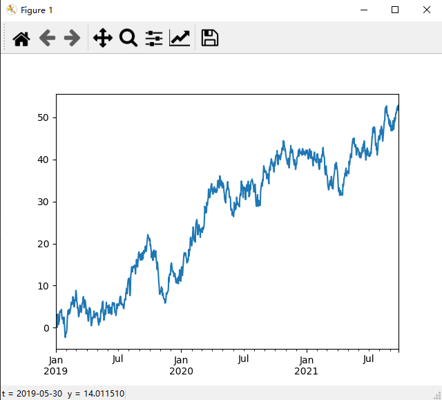
ts = pd.Series(np.random.randn(1000), index=pd.date_range('1/1/2000', periods=1000))
ts = pd.Series(np.random.randn(1000),
index=pd.date_range('1/1/2019', periods=1000))
ts = ts.cumsum()
ts.plot()
Out[182]: <matplotlib.axes._subplots.AxesSubplot at 0x1c318bd80c8>
- DataFrame画图
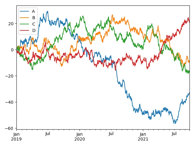
使用plot可以把所有的列都通过标签的形式展示出来:
df = pd.DataFrame(np.random.randn(1000, 4), index=ts.index,
columns=['A', 'B', 'C', 'D'])
df = df.cumsum()
plt.figure()
Out[183]: <Figure size 640x480 with 0 Axes>
df.plot()
Out[184]: <matplotlib.axes._subplots.AxesSubplot at 0x11587e4e0>
plt.legend(loc='best')
导入导出数据 Getting Data In/Out
- CSV
- 写入:
df.to_csv('foo.csv')- 读取:
df.read_csv('foo.csv') - HDF5
- 写入:
df.to_hdf('foo.h5', 'df')- 读取:
pd.read_hdf('foo.h5', 'df') - Excel
- 写入:
df.to_excel('foo.xlsx', sheet_name='Sheet1')- 读取:
pd.read_excel('foo.xlsx', 'Sheet1', index_col=None, na_values=['NA'])
异常处理 Gotchas
如果有一些异常情况比如:
if pd.Series([False, True, False]):
...     print("I was true")
Traceback
    ...
ValueError: The truth value of an array is ambiguous. Use a.empty, a.any() or a.all().

更多推荐


 1
1 0
0- 0


 已为社区贡献1条内容

所有评论(0)