In the previous post we had explored SQL Server Lead Window Function and different examples with use-cases. Next in this post we will be understanding LAG Window Function, its syntax and we will also learn through different examples with use-cases. LAG Window Function is also an analytic function and like LEAD function, its quite similar to LEAD Window Function. It is to be remembered that analytic functions refers to single rows within the window frame and aggregate functions does cumulative operation for all the rows in the window frame. The LAG function gives access to the data of the preceding rows or the row at a given offset that is preceding the current row in the same result set without the use of self-join. in laymans's term it gives us access to the data in the previous rows.'

Syntax

Syntax and its exaplanations is as below, LAG (scalar_expression [,offset] [,default])
OVER ( [ partition_by_clause ] order_by_clause )

scalar_expression: The value to be returned, can be a column name or an expression of any type which returns a single value. It cannot be an analytic function.

offset: It is the value of number of rows preceding the current row from which value is to be obtained, default is 1 if not specified. An offset can be column, subquery, expression returning a positive integer and analytic functions are not allowed.

default: it is the value that can be returned when the offset is outside of the scope f the partition. The default value is null if not specified and it has to be of compatible data type as scalar_expression.

partition_clause: it makes the partitioning or grouping of the dataset as per the criteria mentioned in OVER clause.

order_by: it sorts the data either ascendingly or descendingly before function is applied. If we mention partition by sub-clause, then it will sort the data-set in the partitioning group as per requirement.

Lets prepare a table and dataset for the demonstration.

CREATE TABLE weekly_sales(
    month TINYINT,
    week TINYINT,
    amount DECIMAL(10,2)
);

INSERT INTO weekly_sales(month, week, amount) VALUES 
(1, 1, 35000.00),
(1, 2, 16543.15),
(1, 3, 54453.54),
(1, 4, 45378.12),
(2, 1, 37485.87),
(2, 2, 78567.00),
(2, 3, 54378.00),
(2, 4, 45378.00),
(3, 1, 38753.63),
(3, 2, 23787.03),
(3, 3, 37896.00),
(3, 4, 97855.00);

SQL LAG function without default value

Lets see the simplest implementation of the lag function without default value.

SELECT
    month,
    week,
    amount,
    LAG(amount) OVER(ORDER BY month, week ASC) as lag_amount
FROM weekly_sales;

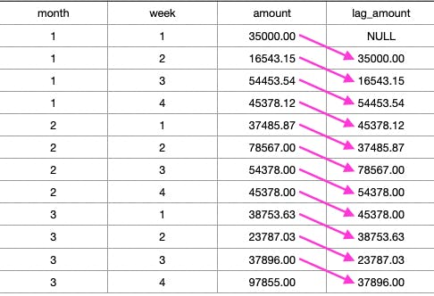
In the above result set it can be seen that the first row have NULL value in lag_amount column as its not in the window frame and rest remaining rows have the value of previous row amount column in its lag_amount column. That is to say that amount of row 1 is set in lag_amount column of row 2 and same pattern follows for all rows.

SQL calculate deltas using LAG function

The LAG() function cam also be usefule like lead function for the analytical calculations like the different between current week sales with previous week sales, cureent week revenue and previous week revenue etc. We will see one example where in along with month, week, amount, we wanted to know previous weeks sales amount and also difference between current week sales with previous week sales.

SELECT
    month,
    week,
    amount as current_sales,
    LAG(amount) OVER(ORDER BY month, week ASC) as previous_week_sales,
    amount - LAG(amount) OVER(ORDER BY month, week ASC) as difference_in_sales
FROM weekly_sales;

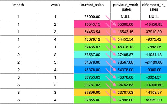
It shows us the difference between the current week sales amount and previous week sales amount, thus highlighting excess or deficit. These types of data are important for analysis for the stakeholders and decision makers.

SQL LAG function example with offset and default value

In the first example query, we havent used the default part and didnt provided the offset value for the lag window function. In this example we will just modify that query to include both the default part and the offset value to refer the previous row. Suppose, we need to generate a report showing the weekly sales of the current week, previous week and the week before the pervious week, we can do it as below.

SELECT
    month,
    week,
    amount as current_week_sales,
    LAG(amount, 1, 0) OVER(ORDER BY month asc, week asc) as previous_week_sales,
    LAG(amount, 2, 0) OVER(ORDER BY month ASC, week ASC) as previous_previous_week_sales
FROM weekly_sales;

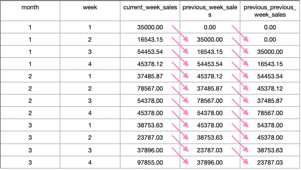
Here in above query we have mentioned both the offset and default value for the lag function. For getting the previous week sales amount we provided offset value as 1 and for getting the week before previous week sales amount we provided offset value of 2. Naturally when the value is not in the scope of the parition then it will return the default value we provided instead of NULL. However the default value and the scalar value should be of the compatible data-type.

SQL LAG function with PARTITION BY and ORDER BY

In all the above examples we didnt provide the PARTITION BY subclause of the OVER clause in the Lag Window Function. So we know if the partition is not provided, it will consider entire dataset of the query as its window frame. Now we wanted to have the data to analyze for the monthly sales

SELECT
    month,
    week,
    amount,
    LAG(amount, 1, 0) OVER(partition by month ORDER BY month ASC, week ASC) as previous_week_sales_amount
FROM weekly_sales;

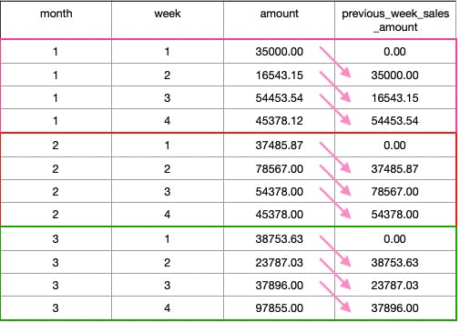
With the lag function we provided the offset value and default value, also since we wanted to analyis the data set month-wise we provided the partition by subclause with the month column. This created three partitioning groups namely month 1, 2 and month 3. In that case the first row;s previous_week_sales_amount value is 0 as it's previous sales amount is out of the scope of the window frame. Similarly we can see that, for the every first row of the month we the previous_week_sales_amount value is 0 as we had partitioned the rowsaet on the basis of the month.'

SQL LAG function with CTE example

The stakeholders or the decision makers wanted to see the report on month to month basis and doesnt want granular data for the weekly sales amount, we can achive the output using the CTE to club/group the sales data base on the months and then we can generate report to show the current month, previous month and the month before the previous month data.

;WITH monthly_sales as (
    SELECT
        month, 
        SUM(amount) as monthly_sales_amount
    FROM weekly_sales
    GROUP BY month
)

SELECT
    monthly_sales_amount as current_month_sales,
    LAG(monthly_sales_amount, 1, 0) OVER(ORDER BY month) as previous_month_sales,
    LAG(monthly_sales_amount, 2, 0) OVER(ORDER BY month) as month_before_previous_sales
FROM monthly_sales;

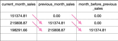
The above query returns the result sets with current month sales, previous month sales and the month before the previous month sales. It return 0 as default value in case of NULL as it's value is out of the Window Frame.' We can use these analytic functions for the generation of data rich and complex reports for the analysis.

Summary

The LAG function gives access to values of the preceding or previous rows as per the offset mentioned, If not mentioned, then the default offset is 1.
PARTITION BY clause sets the local boundary of the data set as per the mentioned specified conditions. If not mentioned, it considers the whole result sets for the boundary.
For out-of-the-frame data, the LAG function returns a NULL value like the LEAD function and we can mention the default value if we want it as a third parameter while calling the function.

In the next post we will be exploring FIRST_VALUE() SQL function.