Human Activity Recognition Using Smartphones Dataset

Dataset : Dataset for this project is downloaded from course website using link below https://d396qusza40orc.cloudfront.net/getdata%2Fprojectfiles%2FUCI%20HAR%20Dataset.zip

Source: The data linked to from the course website represent data collected from the accelerometers from the Samsung Galaxy S smartphone. A full description is available at the site where the data was obtained: http://archive.ics.uci.edu/ml/datasets/Human+Activity+Recognition+Using+Smartphones

Data Set Information:

时间序列数据：按时间顺序记录得数据

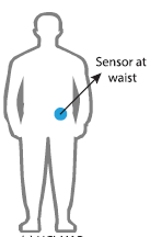
这些数据是从30名年龄在19岁到48岁之间的志愿者身上收集的，这些志愿者将智能手机绑在腰间，进行6项标准活动中的一项，通过开发的手机软件记录运动数据。同时记录每个执行活动的志愿者的视频，后期根据这些视频和传感器数据进行手动标记所属运动类别（类似剪辑视频中的音画同步）。执行的六项活动如下：
Walking；Walking Upstairs；Walking Downstairs；Sitting；Standing；Laying；

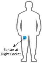
选择30名年龄在19-48岁之间的志愿者作为研究对象。记录的运动数据是来自智能手机（特别是三星Galaxy S II）的x、y和z加速度计数据（线性加速度）和陀螺仪数据（角速度），采样频率为 50Hz（每秒50个数据点）。每名志愿者进行两次活动序列，第一次在设备位于腰间左侧，第二次测试时，智能手机由用户自己按喜好放置。

For each record in the dataset it is provided:

• Triaxial acceleration from the accelerometer (total acceleration) and the estimated body acceleration.
• Triaxial Angular velocity from the gyroscope.
• A 561-feature vector with time and frequency domain variables.
• Its activity label.
• An identifier of the subject who carried out the experiment.

Reference:

1. Davide Anguita, Alessandro Ghio, Luca Oneto, Xavier Parra and Jorge L. Reyes-Ortiz. Human Activity Recognition on Smartphones using a Multiclass Hardware-Friendly Support Vector Machine. International Workshop of Ambient Assisted Living (IWAAL 2012). Vitoria-Gasteiz, Spain. Dec 2012

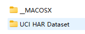
下载的压缩包	解压文件	UCI HAR Dataset

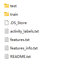（1）UCI HAR Dataset介绍

test：测试集数据；
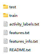train：训练集数据；
activity_labels.txt：活动的真实标签（6个）；
features.txt：特征工程的特征；
features_info.txt：特征工程处理说明；

使用噪声滤波器对加速度计进行预处理。将数据分割成2.56秒（128个数据点）的固定窗口，重叠50%。将加速度计数据分为重力（总）和人体运动分量。

（1）使用中值滤波器和截止频率为 20Hz的三阶低通Butter-worth滤波器对这些信号进行了预处理，以降低噪声。 该速率足以捕获人体运动，因为其能量的99％包含在15Hz以下。

（2）巴特沃斯低通滤波器将具有重力和人体运动成分的加速度信号分离为人体加速度和重力。 假定重力仅具有低频分量，因此从实验中我们发现，对于恒定重力信号，0.3Hz是最佳转折频率。

将特征工程应用于窗口数据，并提供具有这些经过特征工程的数据。从每个窗口中提取了人类活动识别领域中常用的一些时间和频率特征。结果是一个561元素的特征向量。数据集根据受试者的数据分为训练集（70%）和测试集（30%），例如，训练21名受试者，测试9名受试者。

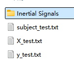
（2）以train文件夹为例，展开叙述：

X_train.txt：未经处理的原始数据，这个不用，可以不关心；(用的是Inertial Signals) y_train.txt：活动类别标签（数字1-6表示），shape为(7352,1)；说明：注意这里的标签是从1开始表示第一类，而one-hot编码是从0开始，注意编码的时候要减去1！这个在以后的建模过程中会遇到，先说明一下。 subject train.txt：将训练集的每一个样本与志愿者编号（1-30）对应，即给每条样本记录属于哪位志愿者做标识，shape为(7352,1)；

（3）以Inertial Signals

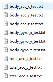
原始数据中有3个主要的类型: total acceleration, body acceleration, and body gyroscope. 每一类有3个维度，也就是说一个时间步有9个变量。此外，每组数据都被划分为2.65秒(128个时间步)的带重叠的窗口。这样每一行就有128*9（1152）个特征，相比于特征工程后的561个特征，显得有些冗余。

body_acc_x_train.txt、body_acc_y_train.txt、body_acc_z_train.txt：三轴的加速度数据； body_gyro_x_train.txt、body_gyro_y_train.txt、body_gyro_z_train.txt：三轴的陀螺仪数据（角速度）； total_acc_x_train.txt、total_acc_y_train.txt、total_acc_z_train.txt：三轴的重力加速度数据；

文件结构：

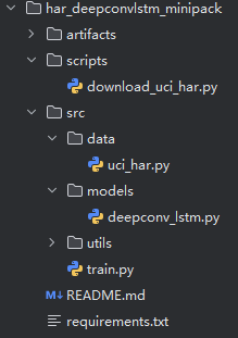其中artifacts文件是模型训练完成后才会出现（保存的权重）。

download_uci_har.py(代码--数据集下载)

#数据集下载
import os
import numpy as np
import torch
from torch.utils.data import Dataset, DataLoader
import matplotlib.pyplot as plt
#导入模块


CHANNEL_FILES = [
    # Order matters: 9 channels (body_acc x/y/z, body_gyro x/y/z, total_acc x/y/z)
    ("body_acc_x", "body_acc_x_train.txt", "body_acc_x_test.txt"),
    ("body_acc_y", "body_acc_y_train.txt", "body_acc_y_test.txt"),
    ("body_acc_z", "body_acc_z_train.txt", "body_acc_z_test.txt"),
    ("body_gyro_x", "body_gyro_x_train.txt", "body_gyro_x_test.txt"),
    ("body_gyro_y", "body_gyro_y_train.txt", "body_gyro_y_test.txt"),
    ("body_gyro_z", "body_gyro_z_train.txt", "body_gyro_z_test.txt"),
    ("total_acc_x", "total_acc_x_train.txt", "total_acc_x_test.txt"),
    ("total_acc_y", "total_acc_y_train.txt", "total_acc_y_test.txt"),
    ("total_acc_z", "total_acc_z_train.txt", "total_acc_z_test.txt"),
]


'''这一行定义了一个名为 _load_split 的函数，接受两个参数：1)root: 数据集的根目录路径（即 UCI HAR Dataset 文件夹的路径）。
2)split: 数据集的子集（文件名称），默认为 "train"，可以传递 "test" 来加载测试集数据。'''
def _load_split(root, split="train"):
    inertial_dir = os.path.join(root, split, "Inertial Signals")    #拼接路径
    assert os.path.isdir(inertial_dir), f"Not found: {inertial_dir}. Did you point to the 'UCI HAR Dataset' folder?"     #assert 语句来检查路径 inertial_dir 是否是一个有效的目录

    # labels  这段代码加载了标签文件
    y_path = os.path.join(root, split, f"y_{split}.txt")
    y = np.loadtxt(y_path, dtype=int)  # 1..6   样本的标签，标签值是 1 到 6 之间的整数。
    y = y - 1  # 0..5    将标签减去 1，使标签变为 0 到 5 之间的整数

    channels = []
    for _, train_file, test_file in CHANNEL_FILES:
        fname = train_file if split == "train" else test_file
        arr = np.loadtxt(os.path.join(inertial_dir, fname))
        channels.append(arr)  # 每个通道的形状为(N, 128)其中 N 是样本的数量（例如，时间窗口的数量）

    X = np.stack(channels, axis=1)  # (N, 9, 128) //np.stack 用于将 9 个信号通道沿新维度
    assert X.shape[0] == y.shape[0], f"X and y size mismatch: {X.shape[0]} vs {y.shape[0]}"
    return X.astype(np.float32), y.astype(np.int64)   #返回 X 和 y。X 是信号数据，y 是标签

class HARWindowDataset(Dataset):
    def __init__(self, X, y, mean=None, std=None):
        self.X = X
        self.y = y
        if mean is None or std is None:
            # compute per-channel statistics across all windows and timesteps (N, C, T)
            '''
            计算每个通道（channel）的均值（mean）和标准差（std），用于后续的标准化操作。'''
            mean = X.mean(axis=(0, 2), keepdims=True)
            std = X.std(axis=(0, 2), keepdims=True) + 1e-8
        self.mean = mean
        self.std = std

    def __len__(self):
        return self.X.shape[0]

    def __getitem__(self, idx):
        # x = (self.X[idx] - self.mean.squeeze()) / self.std.squeeze()
        m = self.mean.squeeze()  # (C,)   每个通道的均值
        s = self.std.squeeze()  # (C,)    每个通道的标准差
        x = (self.X[idx] - m[:, None]) / (s[:, None])  # (C,128) 与 (C,1) 广播    数据标准化（归一化）处理
        return torch.from_numpy(x.astype(np.float32)), torch.tensor(self.y[idx], dtype=torch.long)
        # return torch.from_numpy(x), torch.tensor(self.y[idx])

#加载训练和测试数据集
def make_dataloaders(data_dir, batch_size=64, num_workers=0):
    X_tr, y_tr = _load_split(data_dir, "train")
    X_te, y_te = _load_split(data_dir, "test")

    # Fit stats on train only
    mean = X_tr.mean(axis=(0,2), keepdims=True)
    std = X_tr.std(axis=(0,2), keepdims=True) + 1e-8

    train_ds = HARWindowDataset(X_tr, y_tr, mean, std)
    test_ds  = HARWindowDataset(X_te, y_te, mean, std)

    train_loader = DataLoader(train_ds, batch_size=batch_size, shuffle=True, drop_last=False, num_workers=num_workers)
    test_loader  = DataLoader(test_ds, batch_size=batch_size, shuffle=False, drop_last=False, num_workers=num_workers)

    # Output the first two samples from the training and testing set
    train_iter = iter(train_loader)
    test_iter = iter(test_loader)

    train_data, train_labels = next(train_iter)
    test_data, test_labels = next(test_iter)

    # Get the first two samples
    train_sample_1 = train_data[0], train_labels[0]

    print(f"Train Sample 1: X_shape={train_sample_1[0].shape}.shape, y={train_sample_1[1]}")

    # Output the first channel of the first sample's data (body_acc_x)
    channel_1_data = train_sample_1[0][0]  # Get the first channel (body_acc_x)

    # Plot the first channel's data (body_acc_x)
    plt.figure(figsize=(10, 6))
    plt.plot(channel_1_data.numpy())  # Convert to numpy for plotting
    plt.title('First Sample - First Channel (body_acc_x)')
    plt.xlabel('Time Steps')
    plt.ylabel('Signal Value')
    plt.grid(True)
    plt.show()



    return train_loader, test_loader, mean, std

deepconv_lstm.py(代码）

import torch
import torch.nn as nn
import torch.nn.functional as F
'''引入 PyTorch 基础库与神经网络组件'''


class DeepConvLSTM(nn.Module):
    """
    DeepConvLSTM for HAR
    Input: (B, C, T) where C=9, T=128 for UCI-HAR inertial signals 约定输入张量形状为 (B, C, T)：批量维B、通道数C（UCI-HAR为9个惯导传感通道）、时间步T（UCI-HAR每段长度128）。
    """
    def __init__(self, in_channels=9, n_classes=6, conv_channels=64, n_conv=4,
                 lstm_hidden=128, lstm_layers=1, bidir=False, dropout=0.5):
        super().__init__()
        convs = []
        c_in = in_channels

        '''用于堆叠多个卷积层(conv+BN+ReLU+Dropout).
        n_conv=4 循环的次数
        在每一层卷积后，c_in 更新为当前层的输出通道数 conv_channels，以便在下一层中作为输入通道数。'''
        for i in range(n_conv):
            convs += [
                nn.Conv1d(c_in, conv_channels, kernel_size=5, padding=2),
                nn.BatchNorm1d(conv_channels),
                nn.ReLU(),
                nn.Dropout(dropout),
            ]
            c_in = conv_channels

        self.feat = nn.Sequential(*convs)

        self.lstm = nn.LSTM(
            input_size=conv_channels,
            hidden_size=lstm_hidden,
            num_layers=lstm_layers,
            batch_first=False,
            bidirectional=bidir,
            dropout=dropout if lstm_layers > 1 else 0.0
        )
        #分类头
        out_dim = lstm_hidden * (2 if bidir else 1)
        self.head = nn.Sequential(
            nn.Dropout(dropout),
            nn.Linear(out_dim, n_classes)
        )

    def forward(self, x):  # x: (B,C,T)
        x = self.feat(x)   # (B,F,T)
        x = x.permute(2, 0, 1)  # (T,B,F)
        x, _ = self.lstm(x)     # (T,B,H)
        x = x[-1]               # last time step
        return self.head(x)

train.py(代码）

import os, argparse, time, csv
import numpy as np
import torch
import torch.nn as nn
from sklearn.metrics import accuracy_score, f1_score, classification_report

from models.deepconv_lstm import DeepConvLSTM
from data.uci_har import make_dataloaders
from utils.common import set_seed, count_params, AverageMeter



def train_one_epoch(model, loader, optimizer, device, criterion):
    model.train()
    loss_meter = AverageMeter()
    for xb, yb in loader:
        xb, yb = xb.to(device), yb.to(device)
        optimizer.zero_grad()
        logits = model(xb)
        loss = criterion(logits, yb)
        loss.backward()
        torch.nn.utils.clip_grad_norm_(model.parameters(), 5.0)
        optimizer.step()
        loss_meter.update(loss.item(), xb.size(0))
    return loss_meter.avg

@torch.no_grad()
def evaluate(model, loader, device, criterion):
    model.eval()
    loss_meter = AverageMeter()
    all_y, all_p = [], []
    for xb, yb in loader:
        xb, yb = xb.to(device), yb.to(device)
        logits = model(xb)
        loss = criterion(logits, yb)
        loss_meter.update(loss.item(), xb.size(0))
        probs = torch.softmax(logits, dim=1)
        preds = probs.argmax(dim=1).cpu().numpy()
        all_p.append(preds)
        all_y.append(yb.cpu().numpy())
    all_p = np.concatenate(all_p)
    all_y = np.concatenate(all_y)
    acc = accuracy_score(all_y, all_p)
    f1  = f1_score(all_y, all_p, average="macro")
    return loss_meter.avg, acc, f1, all_y, all_p

def main():
    p = argparse.ArgumentParser()
    p.add_argument("--data_dir", type=str, required=True, help="Path to 'UCI HAR Dataset' folder")
    p.add_argument("--epochs", type=int, default=50)
    p.add_argument("--batch_size", type=int, default=64)
    p.add_argument("--lr", type=float, default=1e-3)
    p.add_argument("--weight_decay", type=float, default=1e-4)
    p.add_argument("--dropout", type=float, default=0.5)
    p.add_argument("--conv_channels", type=int, default=64)
    p.add_argument("--n_conv", type=int, default=4)
    p.add_argument("--lstm_hidden", type=int, default=128)
    p.add_argument("--lstm_layers", type=int, default=1)
    p.add_argument("--bidir", action="store_true")
    p.add_argument("--seed", type=int, default=42)
    p.add_argument("--eval_only", action="store_true")
    p.add_argument("--ckpt_path", type=str, default="artifacts/best_model.pt")
    args = p.parse_args()

    set_seed(args.seed)
    os.makedirs("artifacts", exist_ok=True)
    device = torch.device("cuda" if torch.cuda.is_available() else "cpu")

    # Data
    train_loader, test_loader, mean, std = make_dataloaders(args.data_dir, batch_size=args.batch_size)
    n_classes = 6

    # Model
    model = DeepConvLSTM(
        in_channels=9, n_classes=n_classes, conv_channels=args.conv_channels,
        n_conv=args.n_conv, lstm_hidden=args.lstm_hidden, lstm_layers=args.lstm_layers,
        bidir=args.bidir, dropout=args.dropout
    ).to(device)

    print(f"[info] Params: {count_params(model)/1e6:.2f}M | Device: {device}")

    criterion = nn.CrossEntropyLoss()
    optimizer = torch.optim.Adam(model.parameters(), lr=args.lr, weight_decay=args.weight_decay)
    scheduler = torch.optim.lr_scheduler.ReduceLROnPlateau(optimizer, factor=0.5, patience=5)

    if args.eval_only and os.path.exists(args.ckpt_path):
        model.load_state_dict(torch.load(args.ckpt_path, map_location=device))
        test_loss, test_acc, test_f1, y_true, y_pred = evaluate(model, test_loader, device, criterion)
        print(f"[eval] loss={test_loss:.4f} acc={test_acc:.4f} f1={test_f1:.4f}")
        print(classification_report(y_true, y_pred, digits=4))
        return

    best_f1 = -1.0
    log_path = "artifacts/train_log.csv"
    with open(log_path, "w", newline="") as f:
        w = csv.writer(f)
        w.writerow(["epoch", "train_loss", "val_loss", "val_acc", "val_f1"])

    for epoch in range(1, args.epochs+1):
        tr_loss = train_one_epoch(model, train_loader, optimizer, device, criterion)
        val_loss, val_acc, val_f1, _, _ = evaluate(model, test_loader, device, criterion)
        scheduler.step(val_loss)

        with open(log_path, "a", newline="") as f:
            csv.writer(f).writerow([epoch, f"{tr_loss:.4f}", f"{val_loss:.4f}", f"{val_acc:.4f}", f"{val_f1:.4f}"])

        print(f"[ep {epoch:03d}] train {tr_loss:.4f} | val {val_loss:.4f} acc {val_acc:.4f} f1 {val_f1:.4f}")

        if val_f1 > best_f1:
            best_f1 = val_f1
            torch.save(model.state_dict(), args.ckpt_path)
            print(f"[save] best f1 improved to {best_f1:.4f} -> {args.ckpt_path}")

    # Final evaluation
    model.load_state_dict(torch.load(args.ckpt_path, map_location=device))
    test_loss, test_acc, test_f1, y_true, y_pred = evaluate(model, test_loader, device, criterion)
    print(f"[final] loss={test_loss:.4f} acc={test_acc:.4f} f1={test_f1:.4f}")
    print(classification_report(y_true, y_pred, digits=4))

if __name__ == "__main__":
    main()

代码运行步骤

切换到根目录下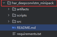（），在运行下面的代码：

python -m  src/train.py --data_dir "./data/UCI HAR Dataset" --epochs 50 --batch_size 64 --lr 1e-3 --weight_decay 1e-4 --dropout 0.5 --bidir

其他参考

UCI-HAR数据集深度剖析：训练仿真与可视化解读-CSDN博客

GitHub - arijitiiest/UCI-Human-Activity-Recognition: Human Activity Recognition Project on UCI-HAR dataset. This model predicts human activities such as Walking, Walking_Upstairs, Walking_Downstairs, Sitting, Standing or Laying. This dataset is collected from 30 persons, performing different activities with a smartphone to their waistshttps://github.com/arijitiiest/UCI-Human-Activity-Recognition?utm_source=chatgpt.com

LSTM-Human-Activity-Recognition/data/source.txt at master · guillaume-chevalier/LSTM-Human-Activity-Recognition · GitHubhttps://github.com/guillaume-chevalier/LSTM-Human-Activity-Recognition/blob/master/data/source.txt

from pandas import read_csv, unique
 
import numpy as np
 
from scipy.interpolate import interp1d
from scipy.stats import mode
 
from sklearn.preprocessing import LabelEncoder
from sklearn.metrics import classification_report, confusion_matrix, ConfusionMatrixDisplay
 
from tensorflow import stack
from tensorflow.keras.utils import to_categorical
from keras.models import Sequential
from keras.layers import Dense, GlobalAveragePooling1D, BatchNormalization, MaxPool1D, Reshape, Activation
from keras.layers import Conv1D, LSTM
from keras.callbacks import ModelCheckpoint, EarlyStopping
import matplotlib.pyplot as plt
%matplotlib inline
 
import warnings
warnings.filterwarnings("ignore")

def read_data(filepath):
    df = read_csv(filepath, header=None, names=['user-id',
                                               'activity',
                                               'timestamp',
                                               'X',
                                               'Y',
                                               'Z'])
    ## removing ';' from last column and converting it to float
    ##在 Z 列中移除了分号（;）
    df['Z'].replace(regex=True, inplace=True, to_replace=r';', value=r'')
    ##将这一列的数据转换为浮点数
    df['Z'] = df['Z'].apply(convert_to_float)
#     df.dropna(axis=0, how='any', inplace=True)
    return df
 
def convert_to_float(x):
    ##转化为float64
    try:
        return np.float64(x)
    except:
        return np.nan
 
df = read_data('Dataset/WISDM_ar_v1.1/WISDM_ar_v1.1_raw.txt')
df

plt.figure(figsize=(15, 5))
 
plt.xlabel('Activity Type')
plt.ylabel('Training examples ')
df['activity'].value_counts().plot(kind='bar',
                                  title='Training examples by Activity Types')
plt.show()##不同活动类型的训练样本数
 
plt.figure(figsize=(15, 5))
plt.xlabel('User')
plt.ylabel('Training examples')
df['user-id'].value_counts().plot(kind='bar', 
                                 title='Training examples by user')
plt.show()##不同活动类型的训练样本数

def axis_plot(ax, x, y, title):
    ax.plot(x, y, 'r')##绘制绘制 x 和 y 数据点，并使用红色（'r'）线条
    ax.set_title(title)
    ax.xaxis.set_visible(False)##隐藏x轴
    ##设置x轴和y轴的范围
    ax.set_ylim([min(y) - np.std(y), max(y) + np.std(y)])
    ax.set_xlim([min(x), max(x)])
    ax.grid(True)
 
for activity in df['activity'].unique():##遍历每种活动类型
    limit = df[df['activity'] == activity][:180]##取前180个
    fig, (ax0, ax1, ax2) = plt.subplots(nrows=3, sharex=True, figsize=(15, 10))
    axis_plot(ax0, limit['timestamp'], limit['X'], 'x-axis')
    axis_plot(ax1, limit['timestamp'], limit['Y'], 'y-axis')
    axis_plot(ax2, limit['timestamp'], limit['Z'], 'z-axis')
    plt.subplots_adjust(hspace=0.2)
    fig.suptitle(activity)
    plt.subplots_adjust(top=0.9)
    plt.show()

label_encode = LabelEncoder()
df['activityEncode'] = label_encode.fit_transform(df['activity'].values.ravel())
df
##将数据框 df 中的 activity 列中的活动类型转换为数字编码，并将结果存储在一个新的列 activityEncode 中

human action recognition-CSDN博客https://blog.csdn.net/qq_56618414/article/details/141817309