决策树完成

平台-- Jupyter Note

ID3方法

主要理论步骤：

ID3：数据集用字典加载，计算熵（用来评估数据的复杂度），计算特征的信息增益（来找到决策树的最佳分支），最后用递归来构建树并打印出来，最后用测试集进行评估
算法实现：

#模块导入
import numpy as np
import pandas as pd
from math import log2
import matplotlib.pyplot as plt
data = {
    'ID': range(1, 17),
    '年龄段': ['青年', '青年', '青年', '青年', '青年', '中年', '中年', '中年', '中年', '中年', 
             '老年', '老年', '老年', '老年', '老年', '老年'],
    '有工作': ['否', '否', '是', '是', '否', '否', '否', '是', '否', '否', 
             '否', '否', '是', '是', '否', '否'],
    '有自己的房子': ['否', '否', '否', '是', '否', '否', '否', '是', '是', '是', 
                  '是', '是', '否', '否', '否', '否'],
    '信贷情况': ['一般', '好', '好', '一般', '一般', '一般', '好', '好', '非常好', '非常好', 
               '非常好', '好', '好', '非常好', '一般', '非常好'],
    '类别(是否给贷款)': ['否', '否', '是', '是', '否', '否', '否', '是', '是', '是', 
                     '是', '是', '是', '是', '否', '否']
}
df=pd.DataFrame(data)

#主体类
class TreeNode:
    def __init__(self, feature=None, value=None, results=None, children=None):
        self.feature = feature      # 分裂特征
        self.value = value          # 特征值
        self.results = results      
        self.children = children or {}  
    
    def is_leaf(self):
        return len(self.children) == 0

def calculate_entropy(labels):
    if len(labels) == 0:
        return 0
    
    value_counts = pd.Series(labels).value_counts()
    entropy_val = 0
    
    for count in value_counts:
        p = count / len(labels)
        entropy_val -= p * log2(p)
    
    return entropy_val

def calculate_information_gain(data, feature, target):
    total_entropy = calculate_entropy(data[target])
    feature_values = data[feature].unique()
    weighted_entropy = 0
    
    for value in feature_values:
        subset = data[data[feature] == value]
        weight = len(subset) / len(data)
        weighted_entropy += weight * calculate_entropy(subset[target])
    
    return total_entropy - weighted_entropy

def build_tree(data, features, target):
    if len(data[target].unique()) == 1:
        return TreeNode(results=data[target].iloc[0])
    
    if len(features) == 0:
        majority_class = data[target].mode()[0]
        return TreeNode(results=majority_class)
    
    best_feature = None
    best_gain = -1
    
    for feature in features:
        gain = calculate_information_gain(data, feature, target)
        if gain > best_gain:
            best_gain = gain
            best_feature = feature
    
    tree = TreeNode(feature=best_feature)
    remaining_features = [f for f in features if f != best_feature]
    
    for value in data[best_feature].unique():
        subset = data[data[best_feature] == value]
        
        if len(subset) == 0:
            majority_class = data[target].mode()[0]
            tree.children[value] = TreeNode#(results=majority_class)
        else:
            tree.children[value] = build_tree(subset, remaining_features, target)
    
    return tree

def predict(tree, sample):
    if tree.is_leaf():
        return tree.results
    
    feature_value = sample[tree.feature]
    if feature_value in tree.children:
        return predict(tree.children[feature_value], sample)
    else:
        return None

# 构建决策树
target_col = '类别(是否给贷款)'
feature_cols = ['年龄段', '有工作', '有自己的房子', '信贷情况']
decision_tree = build_tree(df, feature_cols, target_col)
print("决策树构建完成！")

#加载测试集进行测试

test_data_content = """0,0,0,1,0
0,1,0,1,1
1,0,1,2,1
1,0,0,1,0
2,1,0,2,1
2,0,0,0,0
2,0,0,2,0"""

# 解析测试集数据
test_data = []
for line in test_data_content.strip().split('\n'):
    test_data.append([int(x) for x in line.strip().split(',')])

# 创建测试集DataFrame
test_df = pd.DataFrame(test_data, columns=['年龄段', '有工作', '有自己的房子', '信贷情况', '类别(是否给贷款)'])

# 定义特征映射
age_mapping = {0: '青年', 1: '中年', 2: '老年'}
work_mapping = {0: '否', 1: '是'}
house_mapping = {0: '否', 1: '是'}
credit_mapping = {0: '一般', 1: '好', 2: '非常好'}
class_mapping = {0: '否', 1: '是'}

# 将数字编码转换为原始标签
test_df_decoded = test_df.copy()
test_df_decoded['年龄段'] = test_df['年龄段'].map(age_mapping)
test_df_decoded['有工作'] = test_df['有工作'].map(work_mapping)
test_df_decoded['有自己的房子'] = test_df['有自己的房子'].map(house_mapping)
test_df_decoded['信贷情况'] = test_df['信贷情况'].map(credit_mapping)
test_df_decoded['类别(是否给贷款)'] = test_df['类别(是否给贷款)'].map(class_mapping)

print("测试集数据 (解码后):")
print(test_df_decoded)

predictions = []
for i, row in test_df_decoded.iterrows():
    sample = {
        '年龄段': row['年龄段'],
        '有工作': row['有工作'],
        '有自己的房子': row['有自己的房子'],
        '信贷情况': row['信贷情况']
    }
    prediction = predict(decision_tree, sample)
    predictions.append(prediction)

# 添加预测结果到测试集
test_df_decoded['预测类别'] = predictions

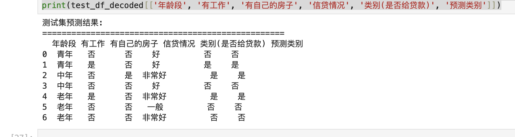
print("测试集预测结果:")
print("=" * 50)
print(test_df_decoded[['年龄段', '有工作', '有自己的房子', '信贷情况', '类别(是否给贷款)', '预测类别']])

def evaluate_predictions(true_labels, predicted_labels):
    correct = 0
    total = len(true_labels)
    
    for true, pred in zip(true_labels, predicted_labels):
        if true == pred:
            correct += 1
    
    accuracy = correct / total
    
    # 计算精确率、召回率和F1分数
    tp = fp = fn = 0
    
    for true, pred in zip(true_labels, predicted_labels):
        if true == '是' and pred == '是':
            tp += 1
        elif true == '否' and pred == '是':
            fp += 1
        elif true == '是' and pred == '否':
            fn += 1
    
    precision = tp / (tp + fp) if (tp + fp) > 0 else 0
    recall = tp / (tp + fn) if (tp + fn) > 0 else 0
    f1 = 2 * precision * recall / (precision + recall) if (precision + recall) > 0 else 0
    
    return accuracy, precision, recall, f1

# 评估模型性能
true_labels = test_df_decoded['类别(是否给贷款)'].tolist()
predicted_labels = test_df_decoded['预测类别'].tolist()

accuracy, precision, recall, f1 = evaluate_predictions(true_labels, predicted_labels)

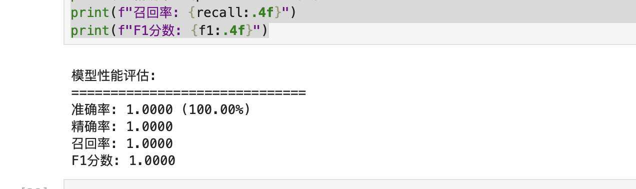
print("\n模型性能评估:")
print("=" * 30)
print(f"准确率: {accuracy:.4f} ({accuracy*100:.2f}%)")
print(f"精确率: {precision:.4f}")
print(f"召回率: {recall:.4f}")
print(f"F1分数: {f1:.4f}")

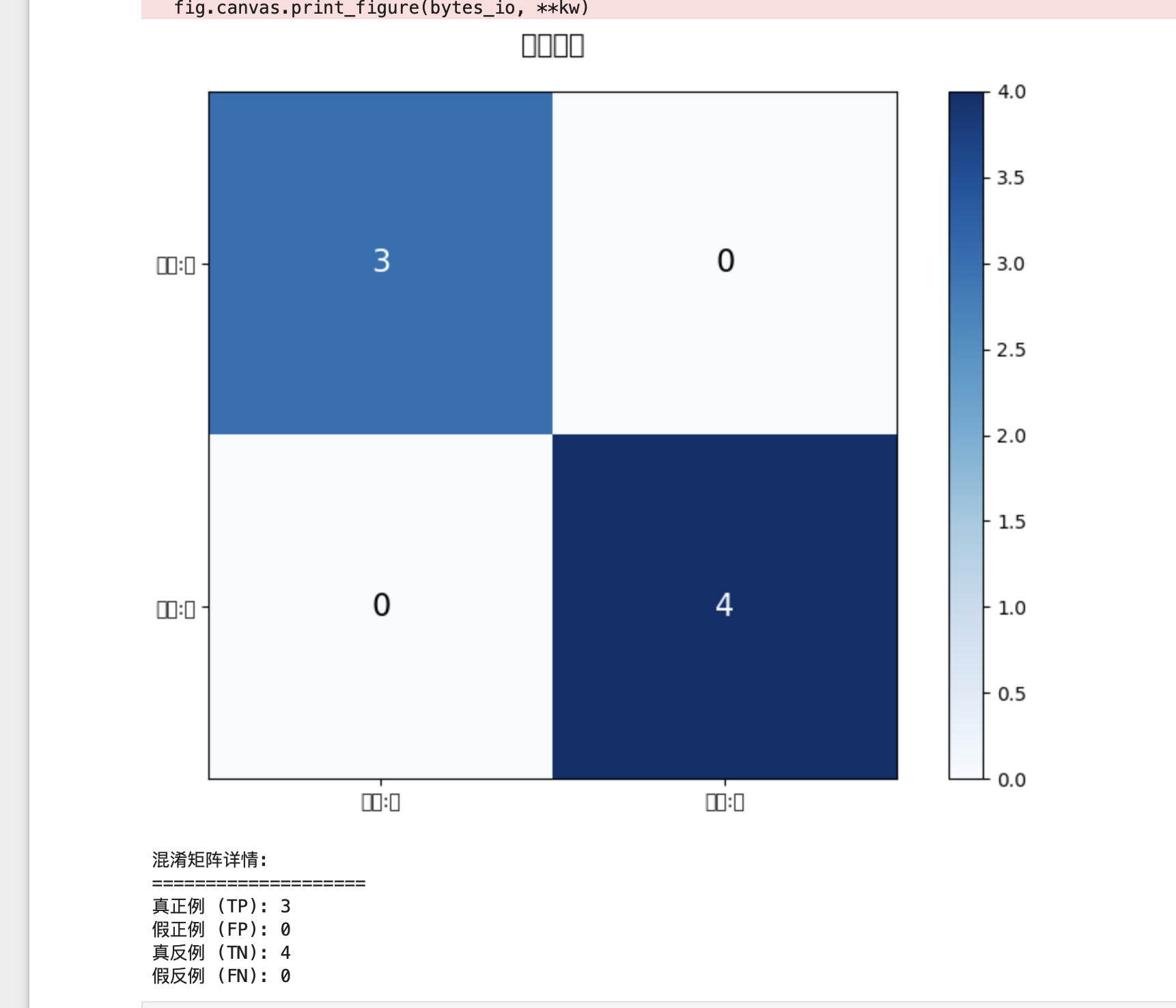
def plot_confusion_matrix(true_labels, predicted_labels):
    cm = {
        ('是', '是'): 0,
        ('是', '否'): 0,
        ('否', '是'): 0,
        ('否', '否'): 0
    }
    
    for true, pred in zip(true_labels, predicted_labels):
        cm[(true, pred)] += 1
    
    # 可视化
    fig, ax = plt.subplots(figsize=(8, 6))
    
    matrix_data = [
        [cm[('是', '是')], cm[('是', '否')]],
        [cm[('否', '是')], cm[('否', '否')]]
    ]
    
    im = ax.imshow(matrix_data, cmap='Blues')
    
    ax.set_xticks([0, 1])
    ax.set_yticks([0, 1])
    ax.set_xticklabels(['预测:是', '预测:否'])
    ax.set_yticklabels(['实际:是', '实际:否'])
    
    for i in range(2):
        for j in range(2):
            ax.text(j, i, str(matrix_data[i][j]), 
                   ha='center', va='center', fontsize=16, 
                   color='white' if matrix_data[i][j] > max(matrix_data[i])/2 else 'black')
    
    plt.title('混淆矩阵', fontsize=14, pad=20)
    plt.colorbar(im)
    plt.tight_layout()
    plt.show()
    
    return cm
 # 绘制混淆矩阵
cm = plot_confusion_matrix(true_labels, predicted_labels)

print("\n混淆矩阵详情:")
print("=" * 20)
print(f"真正例 (TP): {cm[('是', '是')]}")
print(f"假正例 (FP): {cm[('否', '是')]}")
print(f"真反例 (TN): {cm[('否', '否')]}")
print(f"假反例 (FN): {cm[('是', '否')]}")

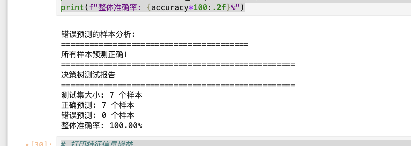
print("\n错误预测的样本分析:")
print("=" * 40)

error_samples = test_df_decoded[test_df_decoded['类别(是否给贷款)'] != test_df_decoded['预测类别']]

if len(error_samples) > 0:
    print("错误预测的样本:")
    for i, row in error_samples.iterrows():
        print(f"样本 {i+1}:")
        print(f"  特征: 年龄段={row['年龄段']}, 有工作={row['有工作']}, 有自己的房子={row['有自己的房子']}, 信贷情况={row['信贷情况']}")
        print(f"  实际类别: {row['类别(是否给贷款)']}")
        print(f"  预测类别: {row['预测类别']}")
        print()
else:
    print("所有样本预测正确！")

# 综合测试报告
print("=" * 50)
print("决策树测试报告")
print("=" * 50)
print(f"测试集大小: {len(test_df)} 个样本")
print(f"正确预测: {len(test_df) - len(error_samples)} 个样本")
print(f"错误预测: {len(error_samples)} 个样本")
print(f"整体准确率: {accuracy*100:.2f}%")

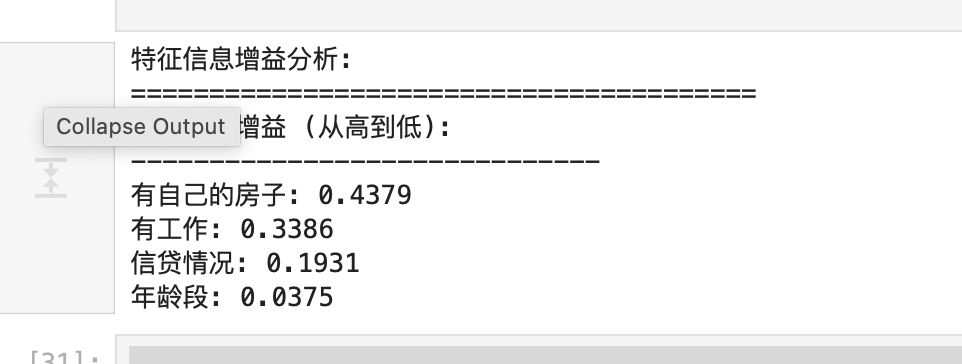
# 打印特征信息增益
print("特征信息增益分析:")
print("=" * 40)

# 重新计算信息增益以确保准确性
target_col = '类别(是否给贷款)'
feature_cols = ['年龄段', '有工作', '有自己的房子', '信贷情况']

# 计算每个特征的信息增益
info_gains = {}
for feature in feature_cols:
    ig = calculate_information_gain(df, feature, target_col)
    info_gains[feature] = ig

# 按信息增益排序
sorted_gains = sorted(info_gains.items(), key=lambda x: x[1], reverse=True)

# 打印信息增益
print("特征信息增益 (从高到低):")
print("-" * 30)
for feature, gain in sorted_gains:
    print(f"{feature}: {gain:.4f}")

# 可视化信息增益
plt.figure(figsize=(10, 6))
features = [item[0] for item in sorted_gains]
gains = [item[1] for item in sorted_gains]

bars = plt.bar(features, gains, color=['#2E8B57', '#4682B4', '#DAA520', '#CD5C5C'])

# 添加数值标签
for bar, gain in zip(bars, gains):
    plt.text(bar.get_x() + bar.get_width()/2, bar.get_height() + 0.001, 
             f'{gain:.4f}', ha='center', va='bottom', fontweight='bold')

plt.xlabel('特征')
plt.ylabel('信息增益')
plt.title('特征信息增益比较')
plt.grid(axis='y', alpha=0.3)
plt.tight_layout()
plt.show()

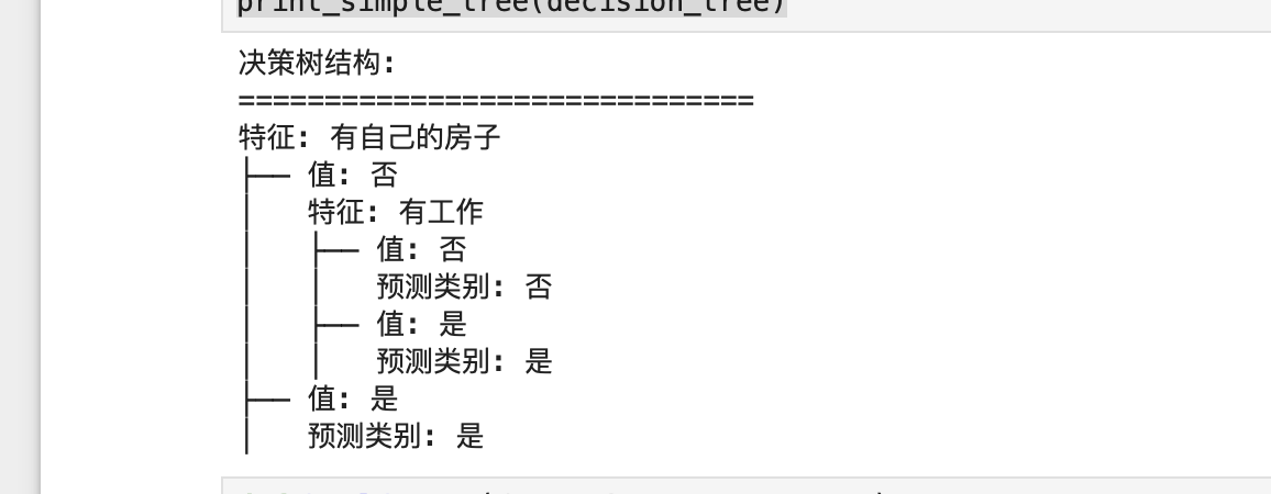
def print_simple_tree(node, indent=""):
    if node.is_leaf():
        print(indent + "预测类别:", node.results)
    else:
        print(indent + "特征:", node.feature)
        for value, child in node.children.items():
            print(indent + "├── 值:", value)
            print_simple_tree(child, indent + "│   ")

print("决策树结构:")
print("=" * 30)
print_simple_tree(decision_tree)

实验结果