1. 为什么需要评估指标？

1. Why do we need evaluation metrics?

训练好一个分类模型后，我们不能只看“预测结果”，而是要知道模型预测对了多少、错在哪里、以及哪种错误更严重。

After training a classification model, we should not only look at the predicted labels. We need to know how many predictions are correct, where the model makes mistakes, and which type of mistake is more costly.

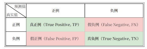
不同应用场景下，错误的代价不同，所以我们需要多种评估指标。

Different applications have different error costs, so we need multiple evaluation metrics.

2. 混淆矩阵：所有指标的根

2. Confusion Matrix: the foundation of all metrics

2.1 猫狗分类例子

2.1 Example: cat vs dog classification

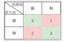
label = ["猫", "狗"]  # labels
y_true = ["猫", "猫", "猫", "猫", "猫", "猫", "狗", "狗", "狗", "狗"]  # ground truth
y_pred = ["猫", "猫", "狗", "猫", "猫", "猫", "猫", "猫", "狗", "狗"]  # predictions

martix = confusion_matrix(y_true, y_pred, labels=label)
print(pd.DataFrame(martix, index=label, columns=label))

2.2 四个关键概念：TP / FP / FN / TN

2.2 Four key terms: TP / FP / FN / TN

我们把“猫”当作正类（pos_label="猫"）。

Assume "cat" is the positive class (pos_label="猫").

• TP（True Positive）：真实是猫，预测也是猫（预测正确的猫）

• TP (True Positive): true cat, predicted cat

• FN（False Negative）：真实是猫，但预测成狗（猫被漏掉了）

• FN (False Negative): true cat, predicted dog (missed cat)

• FP（False Positive）：真实是狗，但预测成猫（把狗误判成猫）

• FP (False Positive): true dog, predicted cat (false alarm)

• TN（True Negative）：真实是狗，预测也是狗（预测正确的狗）

• TN (True Negative): true dog, predicted dog

3. 准确率 Accuracy：整体预测对的比例

3. Accuracy: overall correctness

3.1 公式

3.1 Formula

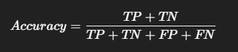
准确率就是“总共预测对了多少”

Accuracy measures “how many predictions are correct overall”.

3.2 生活类比：考试总分

3.2 Life analogy: exam score

Accuracy 就像考试成绩：Accuracy is like an exam score:

你做对了多少题 / 总题数。(number of correct answers) / (total questions).

3.3 Accuracy 的缺点

3.3 Weakness of accuracy

如果类别极度不平衡（比如 99% 都是“狗”），模型只要永远预测“狗”，Accuracy 也会很高，但模型其实没用。

If the dataset is highly imbalanced (e.g., 99% are “dogs”), a model can get high accuracy by always predicting “dog”, even though it is useless.

4. 精确率 Precision：你预测为正的里面有多少是真的？

4. Precision: among predicted positives, how many are truly positive?

4.1 公式

4.1 Formula

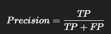
精确率关注：你说“这是猫”的这些样本里，有多少真的是猫。

Precision focuses on: among samples predicted as “cat”, how many are truly cats.
Also called positive predictive value.

4.2 生活类比：抓小偷

4.2 Life analogy: catching thieves

把“猫”当作“小偷”，模型是保安：Treat “cat” as “thief” and the model as a security guard.

你抓出来的人里面，小偷比例越高，Precision 越高。The higher the proportion of real thieves among those caught, the higher the precision.

Precision 高意味着：误抓无辜的人少（FP少）。High precision means fewer innocent people are wrongly accused (low FP).

5. 召回率 Recall：所有真正的正类，你找回了多少？

5. Recall: among all true positives, how many are detected?

5.1 公式

5.1 Formula

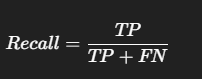
召回率关注：所有真实是猫的样本里，你抓到了多少。

Recall focuses on: among all true cats, how many were detected.

也叫：查全率。Also called sensitivity.

5.2 生活类比：癌症筛查

5.2 Life analogy: cancer screening

把“猫”当作“癌症患者”，模型是筛查系统：

Treat “cat” as “cancer patient” and the model as a screening system.

召回率越高，说明漏诊越少（FN少）。

Higher recall means fewer missed patients (low FN).

医疗筛查更怕 FN（漏检），所以更重视 Recall。

In medical screening, FN is very costly, so recall is often prioritized.

6. Precision 和 Recall 为什么会冲突？

6. Why do precision and recall conflict?

很多模型输出的是概率，而不是直接给类别。

Many models output probabilities, not just labels.

当你调节阈值时，会改变 Precision 和 Recall 的平衡：

Changing the decision threshold trades off precision and recall:

阈值低：更容易判为“猫” → Recall 高，但 FP 变多 → Precision 下降

Low threshold: easier to predict “cat” → high recall, more FP → lower precision

阈值高：更严格才判为“猫” → Precision 高，但 FN 变多 → Recall 下降

High threshold: stricter to predict “cat” → high precision, more FN → lower recall

7. F1-score：Precision 和 Recall 的平衡

7. F1-score: balancing precision and recall

7.1 公式

7.1 Formula

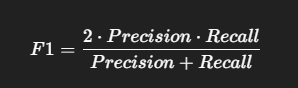
F1 是精确率和召回率的调和平均。

F1 is the harmonic mean of precision and recall.

只要 Precision 或 Recall 有一个很低，F1 就会被拉低。

If either precision or recall is low, F1 will drop significantly.

7.2 生活类比：综合能力评分

7.2 Life analogy: overall performance score

Precision 像“做事准不准”，Recall 像“做事全不全”。

Precision is “how accurate you are”, recall is “how complete you are”.

F1 就像综合评分：既要准，也要全。

F1 is like an overall performance score: you need both.

8. classification_report：一键输出所有指标

8. classification_report: one function for all metrics

report = classification_report(y_true, y_pred, labels=label)
print(report)

它会输出每个类别的 precision、recall、f1-score，还会给出 accuracy、macro avg、weighted avg。

It outputs precision/recall/F1 for each class, plus accuracy, macro average, and weighted average.

from sklearn.metrics import recall_score, confusion_matrix
import pandas as pd
import seaborn as sns

label = ["猫", "狗"]# 标签
y_true = ["猫", "猫", "猫", "猫", "猫", "猫", "狗", "狗", "狗", "狗"] # 真实值
y_pred1 = ["猫", "猫", "狗", "猫", "猫", "猫", "猫", "猫", "狗", "狗"] # 预测值
recall = recall_score(y_true, y_pred1, pos_label="猫")  # pos_label指定正例
print(recall)
martix=confusion_matrix(y_true, y_pred1,labels=label)
print(martix)

print(pd.DataFrame(martix,index=label,columns=label))

#准确率 True Positive + Ture Negative (对的了即可）
from sklearn.metrics import accuracy_score
accuracy=accuracy_score(y_true, y_pred1)#正确预测的比例 TP+FN
print(accuracy)

#热力图
import matplotlib.pyplot as plt
sns.heatmap(martix, annot=True, fmt="d", cmap="YlGn")
plt.show()


#精确率，预测为正例的样本中实际为正例的比例，也叫查准率           抓出来的是对的，降低Flase positive
from sklearn.metrics import precision_score
precision = precision_score(y_true, y_pred1, pos_label="猫")# pos_label指定正例，只算猫
print(precision)

#召回率，实际为正类的样本中预测为正类的比例，也叫查全率
from sklearn.metrics import recall_score    #降低False Negative
recall = recall_score(y_true, y_pred1, pos_label="猫") # pos_label指定正例，只算猫
print(recall)

#F1分数
#精确率和召回率的调和平均
from sklearn.metrics import f1_score
f1 = f1_score(y_true, y_pred1, pos_label="猫")  # pos_label指定正例 只算猫
print(f1)


from sklearn.metrics import classification_report
#评估报告
report=classification_report(y_true, y_pred1, labels=label,target_names=None)    #lables=label默认每个值都要被统计
print(report)

9. 逻辑回归训练 + 评估报告

9.Logistic Regression training + evaluation

• 生成二分类数据集 X, y      Generate a binary dataset X, y

• 划分训练集与测试集                       Split into train/test sets

• 训练逻辑回归模型                           Train a Logistic Regression model

• 预测类别和预测概率                         Predict labels and probabilities

• 输出 classification_report                 Print classification_report

y_pred = model.predict(x_test)p
y_proba = model.predict_proba(x_test)

9.1 predict_proba 为什么重要？

9.1 Why predict_proba matters?

predict() 给出最终类别，predict_proba() 给出概率。

predict() gives the final label, while predict_proba() gives probabilities.
概率代表模型的“信心”，在真实业务中非常重要。

Probabilities represent model confidence and are crucial in real applications.

10. 指标选择：到底应该看哪个？

10. Which metric should you focus on?

10.1 更怕误报（FP） → 看 Precision

10.1 If false alarms are costly (FP) → focus on Precision

• 垃圾邮件过滤（误杀正常邮件很烦）Spam filtering (blocking normal emails is annoying)

• 金融风控（误判正常用户为风险用户）Financial risk control (wrongly flagging normal users)

• 抓小偷（误抓无辜代价高）Catching thieves (wrong accusations are costly)

10.2 更怕漏报（FN） → 看 Recall

10.2 If missed detection is costly (FN) → focus on Recall

• 癌症筛查（漏检很危险）Cancer screening (missing a patient is dangerous)

• 安检危险品识别               Security screening

• 工厂缺陷检测                   Industrial defect detection

10.3 希望平衡 → 看 F1-score

10.3 If you need balance → focus on F1-score

多数普通二分类任务，F1 是很好的综合指标。

For many general binary classification tasks, F1 is a strong overall metric.

from sklearn.datasets import make_classification        #自带的分类数据集
from sklearn.model_selection import train_test_split    #划分数据集
from sklearn.linear_model import LogisticRegression     #逻辑回归
from sklearn.metrics import classification_report        #评估报告

#生成数据集
X, y = make_classification(n_samples=1000, n_features=20, n_classes=2, random_state=100)
#print(X,y)

#1000 行：代表 1000 个样本（1000 条数据）
#20 列：代表每个样本有 20 个特征（20 个输入变量）
#y 是标签（label），也就是模型要预测的答案
#print(X.shape)  # (1000, 20)
#print(y.shape)  # (1000,)
#print(X[0])     # 第1个样本的20个特征
print(y[0:5])     # 第1个样本的标签


# 划分训练集和测试集
x_train, x_test, y_train, y_test = train_test_split(X, y, test_size=0.3, random_state=100)

# 训练一个逻辑回归模型
model = LogisticRegression()
model.fit(x_train, y_train)

#定义分类模型
model = LogisticRegression()

#训练
model.fit(x_train, y_train)

#预测
y_pred = model.predict(x_test)
print(y_pred[0:5])
y_proba=model.predict_proba(x_test)
print(y_proba[0:5])
#哪个概率大就被判定为哪个

#生成评估报告
report = classification_report(y_test, y_pred)
print(report)

11. ROC 曲线与 AUC：模型在不同阈值下的整体区分能力

11. ROC Curve & AUC: overall separability across thresholds

11.1 为什么需要 ROC / AUC？

11.1 Why do we need ROC / AUC?

前面我们讨论了 Accuracy、Precision、Recall、F1。它们都有一个共同点：
它们依赖某一个固定的分类阈值（例如默认阈值 0.5）。

Accuracy, precision, recall, and F1 are all computed under a fixed threshold (often 0.5).

但是在真实任务中，阈值往往需要调整：

However, in real applications, the threshold is adjustable:

• 风控场景：阈值可能设得很高（避免误杀）

• Risk control: high threshold (reduce false alarms)

• 医疗筛查：阈值可能设得很低（尽量不漏检）

• Medical screening: low threshold (reduce missed cases)

ROC 曲线的意义在于：

它不是看某一个阈值下的表现，而是看“所有阈值下”的表现。

ROC evaluates performance across all thresholds, not just one.

11.2 ROC 曲线是什么？

11.2 What is the ROC curve?

ROC 曲线（Receiver Operating Characteristic Curve）是一条曲线，它的横纵坐标是：

ROC (Receiver Operating Characteristic) is a curve with:

• 横轴：FPR（False Positive Rate）假阳性率

• X-axis: FPR (False Positive Rate)

• 纵轴：TPR（True Positive Rate）真正率（也就是 Recall）

• Y-axis: TPR (True Positive Rate) (same as Recall)

11.3 TPR 和 FPR 的公式

11.3 Formulas for TPR and FPR

TPR（真正率 / 召回率）TPR (True Positive Rate / Recall)

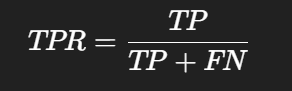
真实为正类的样本中，有多少被预测成正类。

Among all true positives, how many are correctly predicted as positive.

FPR（假阳性率）

FPR (False Positive Rate)

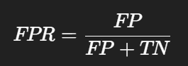
真实为负类的样本中，有多少被误判成正类。

Among all true negatives, how many are incorrectly predicted as positive.

11.4 ROC 曲线怎么来的？

11.4 How is the ROC curve generated?

ROC 曲线通过不断改变阈值来得到。

ROC is generated by sweeping the decision threshold.

例如模型输出概率：

• 如果阈值设为 0.9：只有非常确定的样本才判为正类 → FPR低，TPR可能也低

• Threshold 0.9: very strict → low FPR, but TPR may also drop

• 如果阈值设为 0.1：只要有一点可能就判为正类 → TPR高，但 FPR也高

• Threshold 0.1: very loose → high TPR, but FPR increases

每一个阈值都会产生一个点（FPR, TPR），所有点连起来就是 ROC 曲线。

Each threshold gives one (FPR, TPR) point. Connecting them forms the ROC curve.

11.5 AUC 是什么？为什么越大越好？

11.5 What is AUC and why larger is better?

AUC（Area Under Curve）是 ROC 曲线下的面积：

AUC (Area Under the Curve) is the area under the ROC curve:

模型把正类样本排在负类样本前面的概率

the probability that a random positive sample is ranked higher than a random negative sample.

• AUC = 1.0：完美区分

• AUC = 1.0: perfect separation

• AUC = 0.5：接近随机猜测

• AUC = 0.5: random guessing

• AUC < 0.5：比随机还差（可能预测反了）

• AUC < 0.5: worse than random (maybe reversed labels)

11.6. 代码实现：计算 AUC 并绘制 ROC 曲线

from sklearn.datasets import make_classification        #自带的分类数据集
from sklearn.model_selection import train_test_split    #划分数据集
from sklearn.linear_model import LogisticRegression     #逻辑回归
from sklearn.metrics import classification_report        #评估报告
from sklearn.metrics import roc_auc_score
#AUC值代表ROC曲线下的面积，用于量化模型性能。AUC值越大，模型区分正负类的能力越强，模型性能越好。AUC值=0.5表示模型接近随机猜测.

#生成数据集
X, y = make_classification(n_samples=1000, n_features=20, n_classes=2, random_state=100)
#print(X,y)

#1000 行：代表 1000 个样本（1000 条数据）
#20 列：代表每个样本有 20 个特征（20 个输入变量）
#y 是标签（label），也就是模型要预测的答案
#print(X.shape)  # (1000, 20)
#print(y.shape)  # (1000,)
#print(X[0])     # 第1个样本的20个特征
print(y[0:5])     # 第1个样本的标签


# 划分训练集和测试集
x_train, x_test, y_train, y_test = train_test_split(X, y, test_size=0.3, random_state=100)

# 训练一个逻辑回归模型
model = LogisticRegression()
model.fit(x_train, y_train)

#定义分类模型
model = LogisticRegression()

#训练
model.fit(x_train, y_train)

#预测
y_pred = model.predict(x_test)
print(y_pred[0:5])
y_proba=model.predict_proba(x_test)
print(y_proba[0:5])
#哪个概率大就被判定为哪个

#生成评估报告
report = classification_report(y_test, y_pred)
print(report)

#7计算 ROC AUC
from sklearn.metrics import roc_auc_score
#AUC值代表ROC曲线下的面积，用于量化模型性能。AUC值越大，模型区分正负类的能力越强，模型性能越好。AUC值=0.5表示模型接近随机猜测.
auc=roc_auc_score(y_test,y_proba[:,1])
print(auc)

from sklearn.metrics import roc_curve, auc
import matplotlib.pyplot as plt

# 8 绘制 ROC 曲线
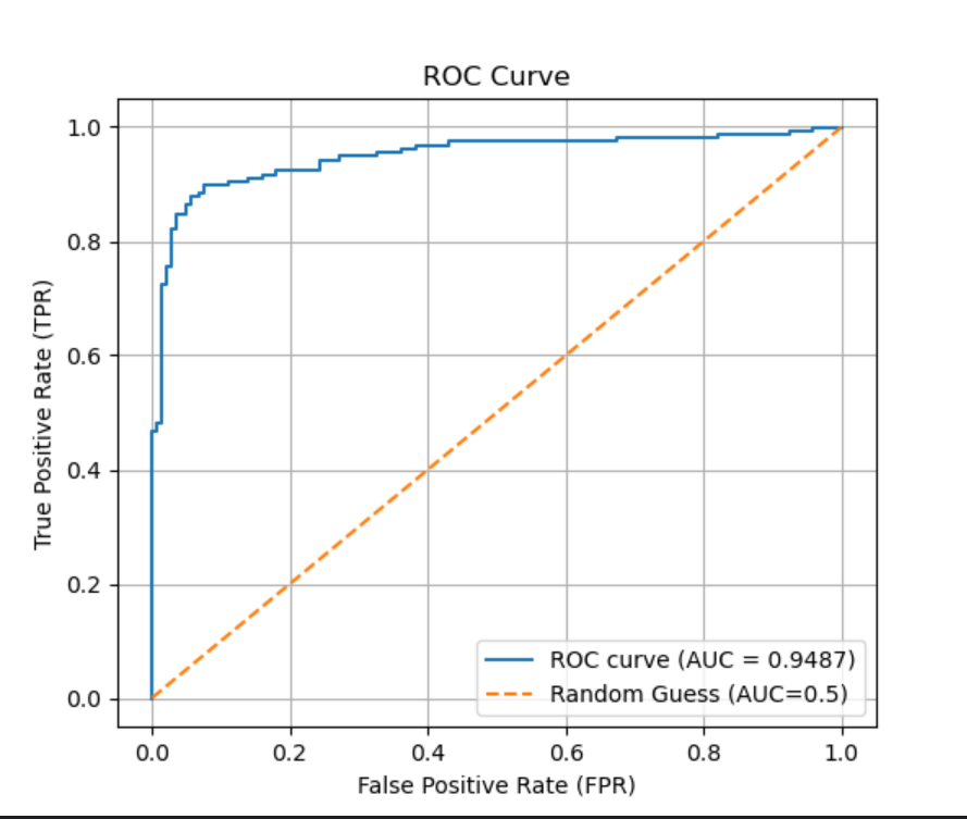
fpr, tpr, thresholds = roc_curve(y_test, y_proba[:, 1])
roc_auc = auc(fpr, tpr)

# 画图
plt.figure(figsize=(6, 5))
plt.plot(fpr, tpr, label=f"ROC curve (AUC = {roc_auc:.4f})")
plt.plot([0, 1], [0, 1], linestyle="--", label="Random Guess (AUC=0.5)")

plt.xlabel("False Positive Rate (FPR)")
plt.ylabel("True Positive Rate (TPR)")
plt.title("ROC Curve")
plt.legend()
plt.grid(True)
plt.show()