
机器学习分类算法一——决策树
一、算法原理
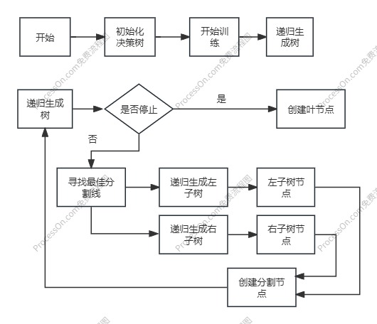
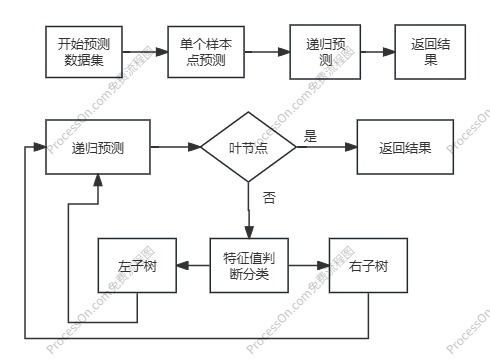
决策树算法通过将数据集划分为不同的子集来预测目标变量。它从根节点开始,根据某个特征对数据集进行划分,然后递归地生成更多的子节点,直到满足停止条件为止。决策树的每个内部节点表示一个特征属性上的判断条件,每个分支代表一个可能的属性值,每个叶节点表示一个分类结果。
二、参考代码
import numpy as np
import matplotlib.pyplot as plt
from matplotlib.patches import Rectangle, FancyArrowPatch


class TreeNode:
    def __init__(self, feature_idx=None, threshold=None, left=None, right=None, class_dist=None):
        self.feature_idx = feature_idx  # 分割特征索引
        self.threshold = threshold      # 分割阈值
        self.left = left                # ≤ threshold 的子树
        self.right = right              # > threshold 的子树
        self.class_dist = class_dist    # 叶子节点的类别分布(用于预测)

class SimpleDecisionTree:
    def __init__(self, max_depth=3):
        self.max_depth = max_depth
        self.tree = None
        self.n_features = None

    def generate_decisiontree_data(self, minn=None, maxx=None, ymin=None, ymax=None, n_samples=1000):
        """
        生成决策树分类数据

        参数:
            minn (list/array): 每个特征的最小值列表,
            maxx (list/array): 每个特征的最大值列表
            ymin (list/array): 标签为1时每个特征的最小值列表
            ymax (list/array): 标签为1时每个特征的最大值列表
            n_samples (int): 生成样本数量,默认为1000

        返回:
            X (ndarray): 特征矩阵 (n_samples,)
            y (ndarray): 标签数组 (n_samples,)
        """
        np.random.seed(42)  # 固定随机种子,确保可复现

        # 设置默认特征范围(年龄和收入)
        if minn is None:
            minn = [0, 0]
        if maxx is None:
            maxx = [100, 100]

        # 设置默认决策边界(标签为1的条件)
        if ymin is None:
            ymin = [60, 60]  # 默认年龄>40且收入>70k时标签为1
        if ymax is None:
            ymax = maxx  # 默认最大值与特征最大值相同

        # 验证输入参数
        if len(minn) != len(maxx) or (ymin is not None and len(minn) != len(ymin)) or (ymax is not None and len(minn) != len(ymax)):
            raise ValueError("minn, maxx, ymin和ymax的长度必须相同")

        n_features = len(minn)

        # 生成特征数据(每个特征在对应的minn和maxx之间)
        X = np.zeros((n_samples, n_features))
        for i in range(n_features):
            X[:, i] = np.random.uniform(minn[i], maxx[i], size=n_samples)

        # 生成标签(基于简单规则:所有特征在ymin和ymax之间时为1,否则为0)
        y = np.ones(n_samples, dtype=int)  # 默认全部为1
        for i in range(n_features):
            y = y & (X[:, i] >= ymin[i]) & (X[:, i] <= ymax[i])

        # 添加一些噪声(让数据不完全可分)
        noise_idx = np.random.choice(n_samples, size=int(0.1 * n_samples), replace=False)
        y[noise_idx] = 1 - y[noise_idx]  # 翻转10%的标签

        return X, y

    def fit(self, X, y):
        y = np.asarray(y).astype(int)  # 确保 y 是整数

        self.n_features = X.shape[1]
        self.tree = self._grow_tree(X, y, depth=0)

    def _grow_tree(self, X, y, depth):
        n_samples, n_features = X.shape
        n_classes = len(np.unique(y))

        # 停止条件:达到最大深度或所有样本属于同一类别
        if depth >= self.max_depth or n_classes == 1:
            class_dist = np.bincount(y, minlength=2)
            return TreeNode(class_dist=class_dist)

        # 寻找最佳分割
        best_feature, best_threshold = self._best_split(X, y)

        # 递归生长左右子树
        left_idx = X[:, best_feature] <= best_threshold
        right_idx = ~left_idx
        left = self._grow_tree(X[left_idx], y[left_idx], depth + 1)
        right = self._grow_tree(X[right_idx], y[right_idx], depth + 1)

        return TreeNode(best_feature, best_threshold, left, right)

    def _best_split(self, X, y):
        best_gini = float('inf')
        best_feature, best_threshold = None, None

        for feature_idx in range(self.n_features):
            thresholds = np.unique(X[:, feature_idx])
            for threshold in thresholds:
                gini = self._gini_impurity(X[:, feature_idx], y, threshold)
                if gini < best_gini:
                    best_gini = gini
                    best_feature = feature_idx
                    best_threshold = threshold

        return best_feature, best_threshold

    def _gini_impurity(self, feature_col, y, threshold):
        left_idx = feature_col <= threshold
        right_idx = ~left_idx

        if np.sum(left_idx) == 0 or np.sum(right_idx) == 0:
            return float('inf')

        left_dist = np.bincount(y[left_idx], minlength=2)
        right_dist = np.bincount(y[right_idx], minlength=2)

        left_prob = left_dist / np.sum(left_dist)
        right_prob = right_dist / np.sum(right_dist)

        gini_left = 1 - np.sum(left_prob ** 2)
        gini_right = 1 - np.sum(right_prob ** 2)

        total_gini = (np.sum(left_idx) * gini_left + np.sum(right_idx) * gini_right) / len(y)
        return total_gini

    def predict(self, X):
        return np.array([self._predict_single(x, self.tree) for x in X])

    def _predict_single(self, x, node):
        if node.feature_idx is None:  # 叶子节点
            return np.argmax(node.class_dist)
        if x[node.feature_idx] <= node.threshold:
            return self._predict_single(x, node.left)
        else:
            return self._predict_single(x, node.right)

    def visualize_tree(self, feature_names=None, class_names=None):
        if feature_names is None:
            feature_names = [f"Feature {i}" for i in range(self.n_features)]
        if class_names is None:
            class_names = ["no", "yes"]

        fig, ax = plt.subplots(figsize=(12, 8))
        ax.set_xlim(0, 1)
        ax.set_ylim(0, 1)
        ax.axis("off")

        # 动态计算树的高度和宽度
        def calc_tree_size(node):
            if node is None:
                return 0, 0
            left_depth, left_width = calc_tree_size(node.left)
            right_depth, right_width = calc_tree_size(node.right)
            depth = max(left_depth, right_depth) + 1
            width = left_width + right_width + 1
            return depth, width

        tree_depth, tree_width = calc_tree_size(self.tree)
        if tree_width == 0:
            tree_width = 1  # 避免除零错误

        # 递归绘制节点(优化布局)
        def _draw_node(node, x, y, width, height, depth):
            node_width = width / tree_width
            node_height = 0.8 / tree_depth  # 调整节点高度
            margin = 0.02  # 节点间距

            if node is None:
                return

            # 绘制节点框
            if node.feature_idx is not None:  # 分割节点
                label = f"{feature_names[node.feature_idx]} ≤ {node.threshold:.1f}"
                color = "lightblue"
            else:  # 叶子节点
                class_idx = np.argmax(node.class_dist)
                n_samples = np.sum(node.class_dist)
                prob = node.class_dist[class_idx] / n_samples
                label = f"{class_names[class_idx]}\n(n={n_samples}"
                color = "lightgreen" if class_idx == 1 else "lightcoral"

            # 绘制矩形节点
            rect = Rectangle(
                (x - node_width/2 + margin, y - node_height/2 + margin),
                width=node_width - 2*margin,
                height=node_height - 2*margin,
                facecolor=color,
                edgecolor="black",
                linewidth=1,
                transform=ax.transAxes
            )
            ax.add_patch(rect)
            ax.text(
                x, y, label,
                ha="center", va="center",
                transform=ax.transAxes,
                fontsize=8
            )

            # 递归绘制子节点
            if node.left or node.right:
                left_width = width * (calc_tree_size(node.left)[1] / tree_width)
                right_width = width * (calc_tree_size(node.right)[1] / tree_width)
                child_y = y - 0.8 / tree_depth  # 子节点垂直位置

                # 绘制左子树
                if node.left:
                    left_x = x - width/2 + left_width/2
                    _draw_node(node.left, left_x, child_y, left_width, height, depth + 1)
                    # 绘制连线
                    arrow = FancyArrowPatch(
                        posA=(x, y - node_height/2),
                        posB=(left_x, child_y + node_height/2),
                        arrowstyle="->",
                        color="gray",
                        shrinkA=5, shrinkB=5,
                        transform=ax.transAxes
                    )
                    ax.add_patch(arrow)

                # 绘制右子树
                if node.right:
                    right_x = x + width/2 - right_width/2
                    _draw_node(node.right, right_x, child_y, right_width, height, depth + 1)
                    # 绘制连线
                    arrow = FancyArrowPatch(
                        posA=(x, y - node_height/2),
                        posB=(right_x, child_y + node_height/2),
                        arrowstyle="->",
                        color="gray",
                        shrinkA=5, shrinkB=5,
                        transform=ax.transAxes
                    )
                    ax.add_patch(arrow)

        # 从顶部开始绘制(根节点在 y=0.9)
        _draw_node(self.tree, x=0.5, y=0.9, width=1, height=1, depth=0)
        plt.tight_layout()
        plt.show()
三、代码分析
1、决策树生成逻辑
2、决策树预测逻辑
3、最佳分割线
def _best_split(self, X, y):
        best_gini = float('inf')
        best_feature, best_threshold = None, None

        for feature_idx in range(self.n_features):
            thresholds = np.unique(X[:, feature_idx])
            for threshold in thresholds:
                gini = self._gini_impurity(X[:, feature_idx], y, threshold)
                if gini < best_gini:
                    best_gini = gini
                    best_feature = feature_idx
                    best_threshold = threshold

        return best_feature, best_threshold

    def _gini_impurity(self, feature_col, y, threshold):
        left_idx = feature_col <= threshold
        right_idx = ~left_idx

        if np.sum(left_idx) == 0 or np.sum(right_idx) == 0:
            return float('inf')

        left_dist = np.bincount(y[left_idx], minlength=2)
        right_dist = np.bincount(y[right_idx], minlength=2)

        left_prob = left_dist / np.sum(left_dist)
        right_prob = right_dist / np.sum(right_dist)

        gini_left = 1 - np.sum(left_prob ** 2)
        gini_right = 1 - np.sum(right_prob ** 2)

        total_gini = (np.sum(left_idx) * gini_left + np.sum(right_idx) * gini_right) / len(y)
        return total_gini
(1)Gini不纯度
定义:Gini 不纯度衡量的是一个数据集中 随机选取两个样本,其类别不一致的概率。
公式:
G
i
n
i
=
1
−
∑
k
=
1
K
p
k
2
Gini =1-\sum_{k=1}^{K}p_k^2
Gini=1−∑k=1Kpk2
其中,其中:K是类别总数(如二分类问题中 K=2)。
p
k
p_k
pk 是第
k类样本在数据集中的比例。
计算步骤:
1)选择一个分割特征和阈值
如age ≤ 40
2)划分数据:
左子集:满足条件的数据(age ≤ 40)。
右子集:不满足条件的数据(age > 40)。
3)计算左右子集的 Gini 不纯度:
对左子集和右子集分别计算 Gini 不纯度。
4)计算加权平均 Gini 不纯度:
T
o
t
e
l
_
G
i
n
i
=
n
l
e
f
t
n
t
o
t
e
l
∗
G
i
n
i
l
e
f
t
+
n
r
i
g
h
t
n
t
o
t
e
l
∗
G
i
n
i
r
i
g
h
t
Totel \_ Gini=\frac{n_{left}}{n_{totel}}*Gini_{left}+\frac{n_{right}}{n_{totel}}*Gini_{right}
Totel_Gini=ntotelnleft∗Ginileft+ntotelnright∗Giniright
其中,
n
r
i
g
h
t
、
n
l
e
f
t
、
n
t
o
t
e
l
n_{right}、n_{left}、n_{totel}
nright、nleft、ntotel分别为左子集、右子集和总集的样本个数。
四、算法评价
1、应用场景
(1)分类问题
应用场景:决策树广泛用于分类任务,例如垃圾邮件识别、客户分类、疾病诊断等。
原因:决策树能够根据特征将数据分割成不同的类别,提供清晰的分类规则。
(2) 回归问题
应用场景:用于预测连续值输出,如房价预测、销售额预测等。
原因:决策树可以分割数据以最小化预测误差,从而提供对连续变量的预测。
(3) 特征选择
应用场景:在数据预处理阶段,用于识别和选择最重要的特征。
原因:决策树通过信息增益、基尼不纯度等指标评估特征的重要性,帮助简化模型。
(4) 数据探索和可视化
应用场景:用于理解数据中的模式和关系,特别是在初步数据分析阶段。
原因:决策树的可视化特性使得数据的分割和决策过程易于理解和解释。
(5) 异常值检测
应用场景:识别数据中的异常点或离群值。
原因:决策树对异常值具有一定的鲁棒性,同时可以通过观察树的分割路径来检测异常模式。
(6)集成方法的基础
应用场景:作为随机森林、梯度提升树等集成方法的基础模型。
原因:决策树的简单性和可扩展性使其成为构建复杂集成模型的理想选择。
(7)多输出任务
应用场景:同时预测多个目标变量。
原因:决策树能够自然地处理多输出问题,提供对多个相关变量的预测。
2、优点
几乎不用数据清洗。其他的工具往往需要data normalization、创建dummy variables等工作。神经网络在训练之前则必须要先归一化,否则会出现效果不好或者出现梯度爆炸/消失。
运算速度快。训练决策树的成本和数据点的数量为对数关系。
可以同时处理连续变量和离散变量。其他的工具常常只能分析一种变量。
利于理解和解释,便于可视化。对于在模型中观察到的现象,我们很容易用逻辑分析进行解释。然而在黑盒模型中(例如人工神经网络),模型的结果很难解释。
可以使用统计检验来验证模型结果,可以检验模型的可靠性。
即使它的假设与实际上产生数据的真实模型不符合,也能有很好的效果。在千奇百怪的实际问题中,决策树模型可能仅仅比一个神经网络专家精心调参出来的模型结果差一点点。对于追求成本和效率的工业界,这就是现金生产力。
3、缺点
决策树模型容易出现过拟合现象,使得模型的泛化能力很低。 但是我们可以通过剪枝、设置每一个叶节点的最小样本数、设置树的最大深度来减小模型的复杂度,从而避免过拟合现象。
决策树的稳定性较低。 对数据集进行很小的改变就可能导致训练出完全不同的树。我们可以通过使用集成算法(随机森林、XGBoost)来解决这个问题。
决策树的计算结果为局部最优,而非全局最优。 如何建立最优的决策树是一个NP-Complete问题,因此目前的决策树学习算法都是基于启发式算法(heuristic algorithms)。例如贪婪算法(greedy algorithms)就是寻找每一个节点的(局部)最优。每一个节点都取到局部最优不能保证最优我们能获得全局最优。我们可以通过使用集成算法(随机森林、XGBoost)来解决这个问题,在集成算法中,特征和样本会在建立每一棵树的时候进行有放回的抽样。
决策树会受到样本不平衡的影响。 我们需要在训练模型之前平衡样本,避免出现某一个类别在dataset中占绝对多数的情况。
4、过拟合现象
训练集准确率飙升:深度增加后,训练集准确率可能接近 100%(每个样本被单独分类)。
测试集准确率下降:对未见过的数据泛化能力变差,导致少数样本分类错误。
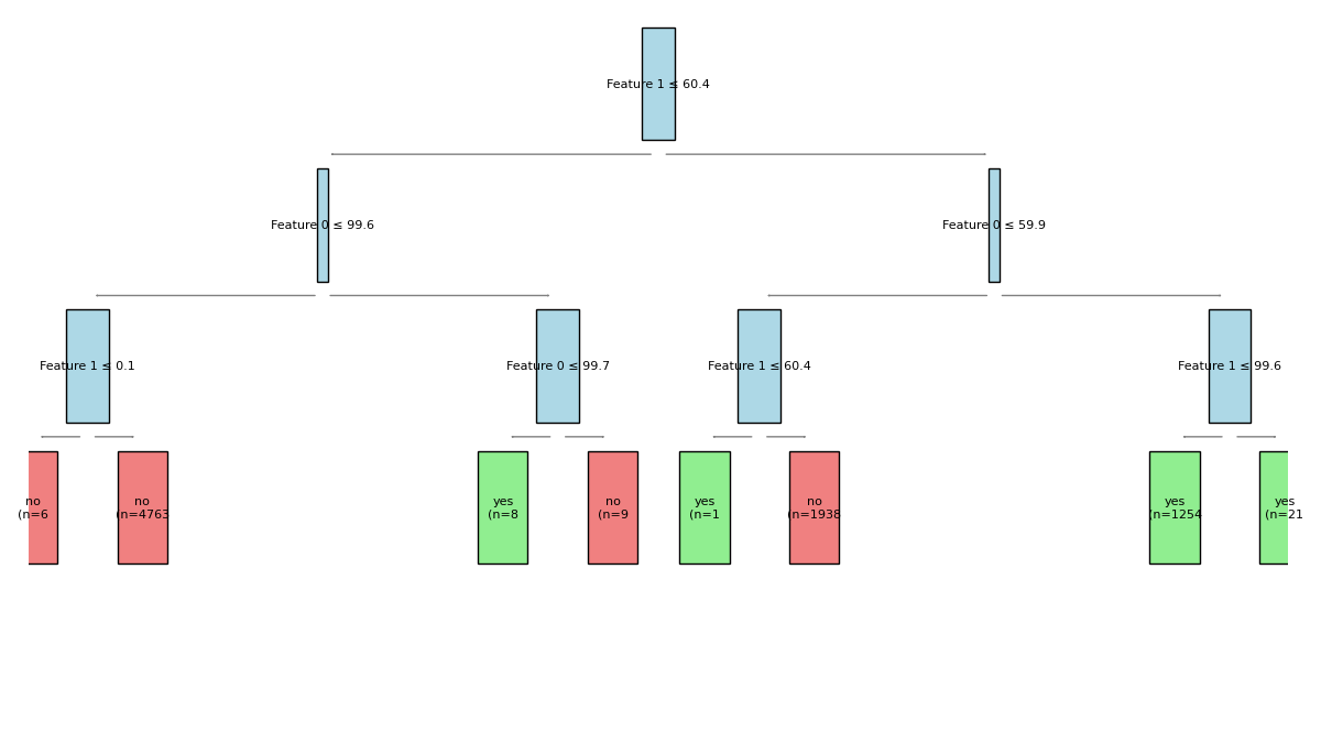
分类边界碎片化:决策边界变得极其复杂,甚至“记住”了噪声或异常值。
在此次实验中,决策树的过拟合现象主要表现在分类边界碎片化,随着深度的增加,出现少数几个点与之前分类不同的现象。
参考文献
更多推荐
 21
21 0
0- 0


 已为社区贡献10条内容

所有评论(0)