
深度学习第P8周:RestNet34实现X光肺炎识别
·
- 🍨 本文为🔗365天深度学习训练营中的学习记录博客
- 🍖 原作者:K同学啊
本周是学习深度学习的第7周。编译器使用的是vscode,安装的是CPU版PyTorch:torch 2.12.0+cpu。
学习目标:
- 跑通RestNet34代码
- 根据官方代码的
结构输出+代码结构图,手动搭建RestNet34算法网络
1 数据集
8530 张胸部 X 光片(正常与肺炎),用于检测肺炎的儿童患者胸部 X 光片(前后)。图像由专家医生进行质量检查和标记;评估集由第三位专家评审。
1.1 导入数据
import os,PIL,random,pathlib

data_dir = './data3/'
data_dir = pathlib.Path(data_dir)

data_paths  = list(data_dir.glob('*'))
classeNames = [str(path).split("\\")[1] for path in data_paths]

# 关于transforms.Compose的更多介绍可以参考:https://blog.csdn.net/qq_38251616/article/details/124878863
train_transforms = transforms.Compose([
    transforms.Resize([224, 224]),  # 将输入图片resize成统一尺寸
    transforms.ToTensor(),          # 将PIL Image或numpy.ndarray转换为tensor,并归一化到[0,1]之间
    transforms.Normalize(           # 标准化处理-->转换为标准正太分布(高斯分布),使模型更容易收敛
        mean=[0.485, 0.456, 0.406],
        std=[0.229, 0.224, 0.225])  # 其中 mean=[0.485,0.456,0.406]与std=[0.229,0.224,0.225] 从数据集中随机抽样计算得到的。
])

test_transform = transforms.Compose([
    transforms.Resize([224, 224]),  # 将输入图片resize成统一尺寸
    transforms.ToTensor(),          # 将PIL Image或numpy.ndarray转换为tensor,并归一化到[0,1]之间
    transforms.Normalize(           # 标准化处理-->转换为标准正太分布(高斯分布),使模型更容易收敛
        mean=[0.485, 0.456, 0.406],
        std=[0.229, 0.224, 0.225])  # 其中 mean=[0.485,0.456,0.406]与std=[0.229,0.224,0.225] 从数据集中随机抽样计算得到的。
])

total_data = datasets.ImageFolder("./data3/",transform=train_transforms)
total_data
此过程输出为:
Dataset ImageFolder
    Number of datapoints: 11807
    Root location: ./data/
    StandardTransform
Transform: Compose(
               Resize(size=[224, 224], interpolation=bilinear, max_size=None, antialias=True)
               ToTensor()
               Normalize(mean=[0.485, 0.456, 0.406], std=[0.229, 0.224, 0.225])
另:
total_data.class_to_idx输出如下结果:
{'NORMAL': 0, 'PNEUMONIA': 1}可以看出数据集有俩类样本。
1.2 数据集划分
train_size = int(0.8 * len(total_data))
test_size  = len(total_data) - train_size
train_dataset, test_dataset = torch.utils.data.random_split(total_data, [train_size, test_size])
train_dataset, test_dataset

batch_size = 64

train_dl = torch.utils.data.DataLoader(train_dataset,
                                       batch_size=batch_size,
                                       shuffle=True,
                                       num_workers=4)
test_dl = torch.utils.data.DataLoader(test_dataset,
                                      batch_size=batch_size,
                                      shuffle=False,
                                      num_workers=4)

for X, y in test_dl:
    print("Shape of X [N, C, H, W]: ", X.shape)
    print("Shape of y: ", y.shape, y.dtype)
    break
输出结果为:
(<torch.utils.data.dataset.Subset at 0x14a45c681a0>,
 <torch.utils.data.dataset.Subset at 0x14a3d205450>)

Shape of X [N, C, H, W]:  torch.Size([64, 3, 224, 224])
Shape of y:  torch.Size([64]) torch.int64
2 模型
本次学习使用了ResNet34 模型。下图为该模型的解释图片:
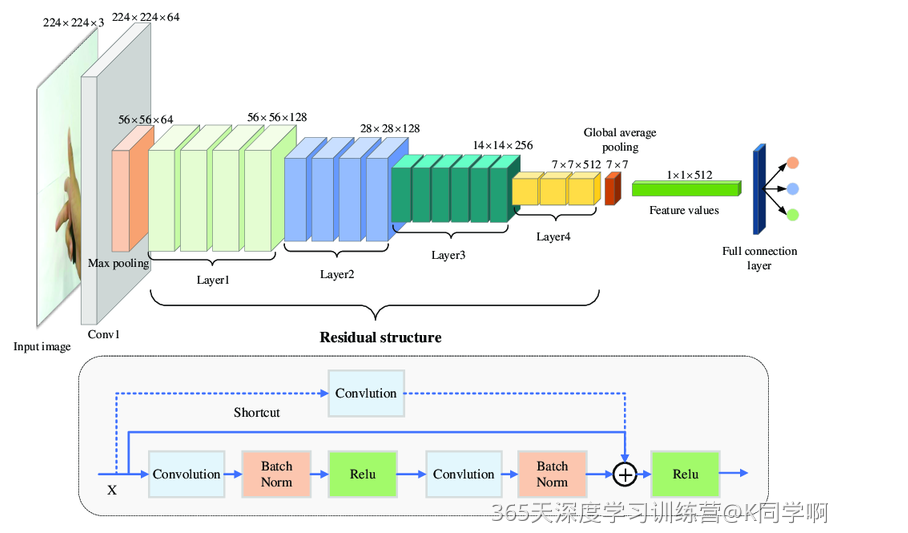
调用模型并查看详情:
from torchvision.models import resnet34

# 加载预训练模型,并且对模型进行微调
model = resnet34(pretrained = True).to(device) # 加载预训练的resnet34模型

for param in model.parameters():
    param.requires_grad = False # 冻结模型的参数,这样子在训练的时候只训练最后一层的参数

# 修改模型的fc层,即(fc): Linear(in_features=512, out_features=2, bias=True)
# 注意查看我们下方打印出来的模型
model.fc = nn.Linear(512,len(classeNames)) # 修改vgg16模型中最后一层全连接层,输出目标类别个数
model.to(device)
model

# 统计模型参数量以及其他指标
import torchsummary as summary
summary.summary(model, (3, 224, 224))
输出结果为:
ResNet(
  (conv1): Conv2d(3, 64, kernel_size=(7, 7), stride=(2, 2), padding=(3, 3), bias=False)
  (bn1): BatchNorm2d(64, eps=1e-05, momentum=0.1, affine=True, track_running_stats=True)
  (relu): ReLU(inplace=True)
  (maxpool): MaxPool2d(kernel_size=3, stride=2, padding=1, dilation=1, ceil_mode=False)
  (layer1): Sequential(
    (0): BasicBlock(
      (conv1): Conv2d(64, 64, kernel_size=(3, 3), stride=(1, 1), padding=(1, 1), bias=False)
      (bn1): BatchNorm2d(64, eps=1e-05, momentum=0.1, affine=True, track_running_stats=True)
      (relu): ReLU(inplace=True)
      (conv2): Conv2d(64, 64, kernel_size=(3, 3), stride=(1, 1), padding=(1, 1), bias=False)
      (bn2): BatchNorm2d(64, eps=1e-05, momentum=0.1, affine=True, track_running_stats=True)
    )
    (1): BasicBlock(
      (conv1): Conv2d(64, 64, kernel_size=(3, 3), stride=(1, 1), padding=(1, 1), bias=False)
      (bn1): BatchNorm2d(64, eps=1e-05, momentum=0.1, affine=True, track_running_stats=True)
      (relu): ReLU(inplace=True)
      (conv2): Conv2d(64, 64, kernel_size=(3, 3), stride=(1, 1), padding=(1, 1), bias=False)
      (bn2): BatchNorm2d(64, eps=1e-05, momentum=0.1, affine=True, track_running_stats=True)
    )
    (2): BasicBlock(
      (conv1): Conv2d(64, 64, kernel_size=(3, 3), stride=(1, 1), padding=(1, 1), bias=False)
      (bn1): BatchNorm2d(64, eps=1e-05, momentum=0.1, affine=True, track_running_stats=True)
      (relu): ReLU(inplace=True)
      (conv2): Conv2d(64, 64, kernel_size=(3, 3), stride=(1, 1), padding=(1, 1), bias=False)
      (bn2): BatchNorm2d(64, eps=1e-05, momentum=0.1, affine=True, track_running_stats=True)
    )
  )
  (layer2): Sequential(
    (0): BasicBlock(
      (conv1): Conv2d(64, 128, kernel_size=(3, 3), stride=(2, 2), padding=(1, 1), bias=False)
      (bn1): BatchNorm2d(128, eps=1e-05, momentum=0.1, affine=True, track_running_stats=True)
      (relu): ReLU(inplace=True)
      (conv2): Conv2d(128, 128, kernel_size=(3, 3), stride=(1, 1), padding=(1, 1), bias=False)
      (bn2): BatchNorm2d(128, eps=1e-05, momentum=0.1, affine=True, track_running_stats=True)
      (downsample): Sequential(
        (0): Conv2d(64, 128, kernel_size=(1, 1), stride=(2, 2), bias=False)
        (1): BatchNorm2d(128, eps=1e-05, momentum=0.1, affine=True, track_running_stats=True)
      )
    )
    (1): BasicBlock(
      (conv1): Conv2d(128, 128, kernel_size=(3, 3), stride=(1, 1), padding=(1, 1), bias=False)
      (bn1): BatchNorm2d(128, eps=1e-05, momentum=0.1, affine=True, track_running_stats=True)
      (relu): ReLU(inplace=True)
      (conv2): Conv2d(128, 128, kernel_size=(3, 3), stride=(1, 1), padding=(1, 1), bias=False)
      (bn2): BatchNorm2d(128, eps=1e-05, momentum=0.1, affine=True, track_running_stats=True)
    )
    (2): BasicBlock(
      (conv1): Conv2d(128, 128, kernel_size=(3, 3), stride=(1, 1), padding=(1, 1), bias=False)
      (bn1): BatchNorm2d(128, eps=1e-05, momentum=0.1, affine=True, track_running_stats=True)
      (relu): ReLU(inplace=True)
      (conv2): Conv2d(128, 128, kernel_size=(3, 3), stride=(1, 1), padding=(1, 1), bias=False)
      (bn2): BatchNorm2d(128, eps=1e-05, momentum=0.1, affine=True, track_running_stats=True)
    )
    (3): BasicBlock(
      (conv1): Conv2d(128, 128, kernel_size=(3, 3), stride=(1, 1), padding=(1, 1), bias=False)
      (bn1): BatchNorm2d(128, eps=1e-05, momentum=0.1, affine=True, track_running_stats=True)
      (relu): ReLU(inplace=True)
      (conv2): Conv2d(128, 128, kernel_size=(3, 3), stride=(1, 1), padding=(1, 1), bias=False)
      (bn2): BatchNorm2d(128, eps=1e-05, momentum=0.1, affine=True, track_running_stats=True)
    )
  )
  (layer3): Sequential(
    (0): BasicBlock(
      (conv1): Conv2d(128, 256, kernel_size=(3, 3), stride=(2, 2), padding=(1, 1), bias=False)
      (bn1): BatchNorm2d(256, eps=1e-05, momentum=0.1, affine=True, track_running_stats=True)
      (relu): ReLU(inplace=True)
      (conv2): Conv2d(256, 256, kernel_size=(3, 3), stride=(1, 1), padding=(1, 1), bias=False)
      (bn2): BatchNorm2d(256, eps=1e-05, momentum=0.1, affine=True, track_running_stats=True)
      (downsample): Sequential(
        (0): Conv2d(128, 256, kernel_size=(1, 1), stride=(2, 2), bias=False)
        (1): BatchNorm2d(256, eps=1e-05, momentum=0.1, affine=True, track_running_stats=True)
      )
    )
    (1): BasicBlock(
      (conv1): Conv2d(256, 256, kernel_size=(3, 3), stride=(1, 1), padding=(1, 1), bias=False)
      (bn1): BatchNorm2d(256, eps=1e-05, momentum=0.1, affine=True, track_running_stats=True)
      (relu): ReLU(inplace=True)
      (conv2): Conv2d(256, 256, kernel_size=(3, 3), stride=(1, 1), padding=(1, 1), bias=False)
      (bn2): BatchNorm2d(256, eps=1e-05, momentum=0.1, affine=True, track_running_stats=True)
    )
    (2): BasicBlock(
      (conv1): Conv2d(256, 256, kernel_size=(3, 3), stride=(1, 1), padding=(1, 1), bias=False)
      (bn1): BatchNorm2d(256, eps=1e-05, momentum=0.1, affine=True, track_running_stats=True)
      (relu): ReLU(inplace=True)
      (conv2): Conv2d(256, 256, kernel_size=(3, 3), stride=(1, 1), padding=(1, 1), bias=False)
      (bn2): BatchNorm2d(256, eps=1e-05, momentum=0.1, affine=True, track_running_stats=True)
    )
    (3): BasicBlock(
      (conv1): Conv2d(256, 256, kernel_size=(3, 3), stride=(1, 1), padding=(1, 1), bias=False)
      (bn1): BatchNorm2d(256, eps=1e-05, momentum=0.1, affine=True, track_running_stats=True)
      (relu): ReLU(inplace=True)
      (conv2): Conv2d(256, 256, kernel_size=(3, 3), stride=(1, 1), padding=(1, 1), bias=False)
      (bn2): BatchNorm2d(256, eps=1e-05, momentum=0.1, affine=True, track_running_stats=True)
    )
    (4): BasicBlock(
      (conv1): Conv2d(256, 256, kernel_size=(3, 3), stride=(1, 1), padding=(1, 1), bias=False)
      (bn1): BatchNorm2d(256, eps=1e-05, momentum=0.1, affine=True, track_running_stats=True)
      (relu): ReLU(inplace=True)
      (conv2): Conv2d(256, 256, kernel_size=(3, 3), stride=(1, 1), padding=(1, 1), bias=False)
      (bn2): BatchNorm2d(256, eps=1e-05, momentum=0.1, affine=True, track_running_stats=True)
    )
    (5): BasicBlock(
      (conv1): Conv2d(256, 256, kernel_size=(3, 3), stride=(1, 1), padding=(1, 1), bias=False)
      (bn1): BatchNorm2d(256, eps=1e-05, momentum=0.1, affine=True, track_running_stats=True)
      (relu): ReLU(inplace=True)
      (conv2): Conv2d(256, 256, kernel_size=(3, 3), stride=(1, 1), padding=(1, 1), bias=False)
      (bn2): BatchNorm2d(256, eps=1e-05, momentum=0.1, affine=True, track_running_stats=True)
    )
  )
  (layer4): Sequential(
    (0): BasicBlock(
      (conv1): Conv2d(256, 512, kernel_size=(3, 3), stride=(2, 2), padding=(1, 1), bias=False)
      (bn1): BatchNorm2d(512, eps=1e-05, momentum=0.1, affine=True, track_running_stats=True)
      (relu): ReLU(inplace=True)
      (conv2): Conv2d(512, 512, kernel_size=(3, 3), stride=(1, 1), padding=(1, 1), bias=False)
      (bn2): BatchNorm2d(512, eps=1e-05, momentum=0.1, affine=True, track_running_stats=True)
      (downsample): Sequential(
        (0): Conv2d(256, 512, kernel_size=(1, 1), stride=(2, 2), bias=False)
        (1): BatchNorm2d(512, eps=1e-05, momentum=0.1, affine=True, track_running_stats=True)
      )
    )
    (1): BasicBlock(
      (conv1): Conv2d(512, 512, kernel_size=(3, 3), stride=(1, 1), padding=(1, 1), bias=False)
      (bn1): BatchNorm2d(512, eps=1e-05, momentum=0.1, affine=True, track_running_stats=True)
      (relu): ReLU(inplace=True)
      (conv2): Conv2d(512, 512, kernel_size=(3, 3), stride=(1, 1), padding=(1, 1), bias=False)
      (bn2): BatchNorm2d(512, eps=1e-05, momentum=0.1, affine=True, track_running_stats=True)
    )
    (2): BasicBlock(
      (conv1): Conv2d(512, 512, kernel_size=(3, 3), stride=(1, 1), padding=(1, 1), bias=False)
      (bn1): BatchNorm2d(512, eps=1e-05, momentum=0.1, affine=True, track_running_stats=True)
      (relu): ReLU(inplace=True)
      (conv2): Conv2d(512, 512, kernel_size=(3, 3), stride=(1, 1), padding=(1, 1), bias=False)
      (bn2): BatchNorm2d(512, eps=1e-05, momentum=0.1, affine=True, track_running_stats=True)
    )
  )
  (avgpool): AdaptiveAvgPool2d(output_size=(1, 1))
  (fc): Linear(in_features=512, out_features=2, bias=True)
)
----------------------------------------------------------------
Layer (type) Output Shape Param #
================================================================
Conv2d-1 [-1, 64, 112, 112] 9,408
BatchNorm2d-2 [-1, 64, 112, 112] 128
ReLU-3 [-1, 64, 112, 112] 0
MaxPool2d-4 [-1, 64, 56, 56] 0
Conv2d-5 [-1, 64, 56, 56] 36,864
BatchNorm2d-6 [-1, 64, 56, 56] 128
ReLU-7 [-1, 64, 56, 56] 0
Conv2d-8 [-1, 64, 56, 56] 36,864
BatchNorm2d-9 [-1, 64, 56, 56] 128
ReLU-10 [-1, 64, 56, 56] 0
BasicBlock-11 [-1, 64, 56, 56] 0
Conv2d-12 [-1, 64, 56, 56] 36,864
BatchNorm2d-13 [-1, 64, 56, 56] 128
ReLU-14 [-1, 64, 56, 56] 0
Conv2d-15 [-1, 64, 56, 56] 36,864
BatchNorm2d-16 [-1, 64, 56, 56] 128
ReLU-17 [-1, 64, 56, 56] 0
BasicBlock-18 [-1, 64, 56, 56] 0
Conv2d-19 [-1, 64, 56, 56] 36,864
BatchNorm2d-20 [-1, 64, 56, 56] 128
ReLU-21 [-1, 64, 56, 56] 0
Conv2d-22 [-1, 64, 56, 56] 36,864
BatchNorm2d-23 [-1, 64, 56, 56] 128
ReLU-24 [-1, 64, 56, 56] 0
BasicBlock-25 [-1, 64, 56, 56] 0
Conv2d-26 [-1, 128, 28, 28] 73,728
BatchNorm2d-27 [-1, 128, 28, 28] 256
ReLU-28 [-1, 128, 28, 28] 0
Conv2d-29 [-1, 128, 28, 28] 147,456
BatchNorm2d-30 [-1, 128, 28, 28] 256
Conv2d-31 [-1, 128, 28, 28] 8,192
BatchNorm2d-32 [-1, 128, 28, 28] 256
ReLU-33 [-1, 128, 28, 28] 0
BasicBlock-34 [-1, 128, 28, 28] 0
Conv2d-35 [-1, 128, 28, 28] 147,456
BatchNorm2d-36 [-1, 128, 28, 28] 256
ReLU-37 [-1, 128, 28, 28] 0
Conv2d-38 [-1, 128, 28, 28] 147,456
BatchNorm2d-39 [-1, 128, 28, 28] 256
ReLU-40 [-1, 128, 28, 28] 0
BasicBlock-41 [-1, 128, 28, 28] 0
Conv2d-42 [-1, 128, 28, 28] 147,456
BatchNorm2d-43 [-1, 128, 28, 28] 256
ReLU-44 [-1, 128, 28, 28] 0
Conv2d-45 [-1, 128, 28, 28] 147,456
BatchNorm2d-46 [-1, 128, 28, 28] 256
ReLU-47 [-1, 128, 28, 28] 0
BasicBlock-48 [-1, 128, 28, 28] 0
Conv2d-49 [-1, 128, 28, 28] 147,456
BatchNorm2d-50 [-1, 128, 28, 28] 256
ReLU-51 [-1, 128, 28, 28] 0
Conv2d-52 [-1, 128, 28, 28] 147,456
BatchNorm2d-53 [-1, 128, 28, 28] 256
ReLU-54 [-1, 128, 28, 28] 0
BasicBlock-55 [-1, 128, 28, 28] 0
Conv2d-56 [-1, 256, 14, 14] 294,912
BatchNorm2d-57 [-1, 256, 14, 14] 512
ReLU-58 [-1, 256, 14, 14] 0
Conv2d-59 [-1, 256, 14, 14] 589,824
BatchNorm2d-60 [-1, 256, 14, 14] 512
Conv2d-61 [-1, 256, 14, 14] 32,768
BatchNorm2d-62 [-1, 256, 14, 14] 512
ReLU-63 [-1, 256, 14, 14] 0
BasicBlock-64 [-1, 256, 14, 14] 0
Conv2d-65 [-1, 256, 14, 14] 589,824
BatchNorm2d-66 [-1, 256, 14, 14] 512
ReLU-67 [-1, 256, 14, 14] 0
Conv2d-68 [-1, 256, 14, 14] 589,824
BatchNorm2d-69 [-1, 256, 14, 14] 512
ReLU-70 [-1, 256, 14, 14] 0
BasicBlock-71 [-1, 256, 14, 14] 0
Conv2d-72 [-1, 256, 14, 14] 589,824
BatchNorm2d-73 [-1, 256, 14, 14] 512
ReLU-74 [-1, 256, 14, 14] 0
Conv2d-75 [-1, 256, 14, 14] 589,824
BatchNorm2d-76 [-1, 256, 14, 14] 512
ReLU-77 [-1, 256, 14, 14] 0
BasicBlock-78 [-1, 256, 14, 14] 0
Conv2d-79 [-1, 256, 14, 14] 589,824
BatchNorm2d-80 [-1, 256, 14, 14] 512
ReLU-81 [-1, 256, 14, 14] 0
Conv2d-82 [-1, 256, 14, 14] 589,824
BatchNorm2d-83 [-1, 256, 14, 14] 512
ReLU-84 [-1, 256, 14, 14] 0
BasicBlock-85 [-1, 256, 14, 14] 0
Conv2d-86 [-1, 256, 14, 14] 589,824
BatchNorm2d-87 [-1, 256, 14, 14] 512
ReLU-88 [-1, 256, 14, 14] 0
Conv2d-89 [-1, 256, 14, 14] 589,824
BatchNorm2d-90 [-1, 256, 14, 14] 512
ReLU-91 [-1, 256, 14, 14] 0
BasicBlock-92 [-1, 256, 14, 14] 0
Conv2d-93 [-1, 256, 14, 14] 589,824
BatchNorm2d-94 [-1, 256, 14, 14] 512
ReLU-95 [-1, 256, 14, 14] 0
Conv2d-96 [-1, 256, 14, 14] 589,824
BatchNorm2d-97 [-1, 256, 14, 14] 512
ReLU-98 [-1, 256, 14, 14] 0
BasicBlock-99 [-1, 256, 14, 14] 0
Conv2d-100 [-1, 512, 7, 7] 1,179,648
BatchNorm2d-101 [-1, 512, 7, 7] 1,024
ReLU-102 [-1, 512, 7, 7] 0
Conv2d-103 [-1, 512, 7, 7] 2,359,296
BatchNorm2d-104 [-1, 512, 7, 7] 1,024
Conv2d-105 [-1, 512, 7, 7] 131,072
BatchNorm2d-106 [-1, 512, 7, 7] 1,024
ReLU-107 [-1, 512, 7, 7] 0
BasicBlock-108 [-1, 512, 7, 7] 0
Conv2d-109 [-1, 512, 7, 7] 2,359,296
BatchNorm2d-110 [-1, 512, 7, 7] 1,024
ReLU-111 [-1, 512, 7, 7] 0
Conv2d-112 [-1, 512, 7, 7] 2,359,296
BatchNorm2d-113 [-1, 512, 7, 7] 1,024
ReLU-114 [-1, 512, 7, 7] 0
BasicBlock-115 [-1, 512, 7, 7] 0
Conv2d-116 [-1, 512, 7, 7] 2,359,296
BatchNorm2d-117 [-1, 512, 7, 7] 1,024
ReLU-118 [-1, 512, 7, 7] 0
Conv2d-119 [-1, 512, 7, 7] 2,359,296
BatchNorm2d-120 [-1, 512, 7, 7] 1,024
ReLU-121 [-1, 512, 7, 7] 0
BasicBlock-122 [-1, 512, 7, 7] 0
AdaptiveAvgPool2d-123 [-1, 512, 1, 1] 0
Linear-124 [-1, 2] 1,026
================================================================
Total params: 21,285,698
Trainable params: 1,026
Non-trainable params: 21,284,672
----------------------------------------------------------------
Input size (MB): 0.57
Forward/backward pass size (MB): 96.28
Params size (MB): 81.20
Estimated Total Size (MB): 178.05
----------------------------------------------------------------3 模型训练与可视化
3.1 训练函数与测试函数
# 训练循环
def train(dataloader, model, loss_fn, optimizer):
    size = len(dataloader.dataset)  # 训练集的大小
    num_batches = len(dataloader)   # 批次数目, (size/batch_size,向上取整)

    train_loss, train_acc = 0, 0  # 初始化训练损失和正确率

    for X, y in dataloader:  # 获取图片及其标签
        X, y = X.to(device), y.to(device)

        # 计算预测误差
        pred = model(X)          # 网络输出
        loss = loss_fn(pred, y)  # 计算网络输出和真实值之间的差距,targets为真实值,计算二者差值即为损失

        # 反向传播
        optimizer.zero_grad()  # grad属性归零
        loss.backward()        # 反向传播
        optimizer.step()       # 每一步自动更新

        # 记录acc与loss
        train_acc  += (pred.argmax(1) == y).type(torch.float).sum().item()
        train_loss += loss.item()

    train_acc  /= size
    train_loss /= num_batches

    return train_acc, train_loss
测试函数和训练函数大致相同,但是由于不进行梯度下降对网络权重进行更新,所以不需要传入优化器
def test (dataloader, model, loss_fn):
    size        = len(dataloader.dataset)  # 测试集的大小
    num_batches = len(dataloader)          # 批次数目, (size/batch_size,向上取整)
    test_loss, test_acc = 0, 0

    # 当不进行训练时,停止梯度更新,节省计算内存消耗
    with torch.no_grad():
        for X, y in dataloader:
            X, y = X.to(device), y.to(device)

            # 计算loss
            y_pred = model(X)
            loss   = loss_fn(y_pred, y)

            test_loss += loss.item()
            test_acc  += (y_pred.argmax(1) == y).type(torch.float).sum().item()

    test_acc  /= size
    test_loss /= num_batches

    return test_acc, test_loss
3.2 进行正式训练与可视化
import copy

optimizer  = torch.optim.Adam(model.parameters(), lr= 1e-4)
loss_fn    = nn.CrossEntropyLoss() # 创建损失函数

epochs     = 10
train_loss = []
train_acc  = []
test_loss  = []
test_acc   = []

best_acc = 0    # 设置一个最佳准确率,作为最佳模型的判别指标

for epoch in range(epochs):

    model.train()
    epoch_train_acc, epoch_train_loss = train(train_dl, model, loss_fn, optimizer)

    model.eval()
    epoch_test_acc, epoch_test_loss = test(test_dl, model, loss_fn)

    # 保存最佳模型到 best_model
    if epoch_test_acc > best_acc:
        best_acc   = epoch_test_acc
        best_model = copy.deepcopy(model)

    train_acc.append(epoch_train_acc)
    train_loss.append(epoch_train_loss)
    test_acc.append(epoch_test_acc)
    test_loss.append(epoch_test_loss)

    # 获取当前的学习率
    lr = optimizer.state_dict()['param_groups'][0]['lr']

    template = ('Epoch:{:2d}, Train_acc:{:.1f}%, Train_loss:{:.3f}, Test_acc:{:.1f}%, Test_loss:{:.3f}, Lr:{:.2E}')
    print(template.format(epoch+1, epoch_train_acc*100, epoch_train_loss,
                          epoch_test_acc*100, epoch_test_loss, lr))

# 保存最佳模型到文件中
PATH = './best_model.pth'  # 保存的参数文件名
torch.save(best_model.state_dict(), PATH)

print('Done')
可视化部分:
import matplotlib.pyplot as plt
#隐藏警告
import warnings
warnings.filterwarnings("ignore")               #忽略警告信息
plt.rcParams['font.sans-serif']    = ['SimHei'] # 用来正常显示中文标签
plt.rcParams['axes.unicode_minus'] = False      # 用来正常显示负号
plt.rcParams['figure.dpi']         = 100        #分辨率

from datetime import datetime
current_time = datetime.now() # 获取当前时间

epochs_range = range(epochs)

plt.figure(figsize=(12, 3))
plt.subplot(1, 2, 1)

plt.plot(epochs_range, train_acc, label='Training Accuracy')
plt.plot(epochs_range, test_acc, label='Test Accuracy')
plt.legend(loc='lower right')
plt.title('Training and Validation Accuracy')
plt.xlabel(current_time) # 打卡请带上时间戳,否则代码截图无效

plt.subplot(1, 2, 2)
plt.plot(epochs_range, train_loss, label='Training Loss')
plt.plot(epochs_range, test_loss, label='Test Loss')
plt.legend(loc='upper right')
plt.title('Training and Validation Loss')
plt.show()
3.3 结果分析
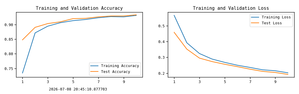
训练过程数据:
Epoch: 1, Train_acc:73.4%, Train_loss:0.565, Test_acc:84.8%, Test_loss:0.458, Lr:1.00E-04
Epoch: 2, Train_acc:87.2%, Train_loss:0.392, Test_acc:89.1%, Test_loss:0.352, Lr:1.00E-04
Epoch: 3, Train_acc:89.5%, Train_loss:0.324, Test_acc:90.4%, Test_loss:0.295, Lr:1.00E-04
Epoch: 4, Train_acc:90.7%, Train_loss:0.289, Test_acc:91.0%, Test_loss:0.273, Lr:1.00E-04
Epoch: 5, Train_acc:91.4%, Train_loss:0.268, Test_acc:92.1%, Test_loss:0.256, Lr:1.00E-04
Epoch: 6, Train_acc:91.8%, Train_loss:0.250, Test_acc:92.2%, Test_loss:0.241, Lr:1.00E-04
Epoch: 7, Train_acc:92.4%, Train_loss:0.236, Test_acc:92.7%, Test_loss:0.225, Lr:1.00E-04
Epoch: 8, Train_acc:92.8%, Train_loss:0.221, Test_acc:93.0%, Test_loss:0.211, Lr:1.00E-04
Epoch: 9, Train_acc:92.7%, Train_loss:0.215, Test_acc:93.0%, Test_loss:0.204, Lr:1.00E-04
Epoch: 10, Train_acc:93.2%, Train_loss:0.202, Test_acc:93.4%, Test_loss:0.192, Lr:1.00E-04
Done
结果图为:
3.4 模型评估
best_model.eval()
epoch_test_acc, epoch_test_loss = test(test_dl, best_model, loss_fn)

epoch_test_acc, epoch_test_loss
输出结果为:
(0.9341687552213868, 0.1918436723947526)4 个人总结
本次学习需要进行手动搭建模型的环节。
RestNet34模型结构代码为:
# 基本残差块
class ResidualBlock(nn.Module):
    def __init__(self, in_channels, out_channels, stride=1):
        super(ResidualBlock, self).__init__()

        self.conv1 = nn.Conv2d(
            in_channels,
            out_channels,
            kernel_size=3,
            stride=stride,
            padding=1,
            bias=False
        )
        self.bn1 = nn.BatchNorm2d(out_channels)
        self.relu = nn.ReLU()

        self.conv2 = nn.Conv2d(
            out_channels,
            out_channels,
            kernel_size=3,
            stride=1,
            padding=1,
            bias=False
        )
        self.bn2 = nn.BatchNorm2d(out_channels)

        # 尺寸或通道数发生变化时,调整残差边的尺寸
        if stride != 1 or in_channels != out_channels:
            self.shortcut = nn.Sequential(
                nn.Conv2d(
                    in_channels,
                    out_channels,
                    kernel_size=1,
                    stride=stride,
                    bias=False
                ),
                nn.BatchNorm2d(out_channels)
            )
        else:
            self.shortcut = nn.Identity()

    def forward(self, x):
        residual = self.shortcut(x)

        x = self.conv1(x)
        x = self.bn1(x)
        x = self.relu(x)

        x = self.conv2(x)
        x = self.bn2(x)

        x = x + residual
        x = self.relu(x)

        return x


class resnet34(nn.Module):
    def __init__(self):
        super(resnet34, self).__init__()

        # 输入层:224×224×3 -> 56×56×64
        self.conv1 = nn.Sequential(
            nn.Conv2d(
                3,
                64,
                kernel_size=7,
                stride=2,
                padding=3,
                bias=False
            ),
            nn.BatchNorm2d(64),
            nn.ReLU(),
            nn.MaxPool2d(
                kernel_size=3,
                stride=2,
                padding=1
            )
        )

        # 残差块1:3个残差单元
        # 输出尺寸:56×56×64
        self.block1 = nn.Sequential(
            ResidualBlock(64, 64),
            ResidualBlock(64, 64),
            ResidualBlock(64, 64)
        )

        # 残差块2:4个残差单元
        # 输出尺寸:28×28×128
        self.block2 = nn.Sequential(
            ResidualBlock(64, 128, stride=2),
            ResidualBlock(128, 128),
            ResidualBlock(128, 128),
            ResidualBlock(128, 128)
        )

        # 残差块3:6个残差单元
        # 输出尺寸:14×14×256
        self.block3 = nn.Sequential(
            ResidualBlock(128, 256, stride=2),
            ResidualBlock(256, 256),
            ResidualBlock(256, 256),
            ResidualBlock(256, 256),
            ResidualBlock(256, 256),
            ResidualBlock(256, 256)
        )

        # 残差块4:3个残差单元
        # 输出尺寸:7×7×512
        self.block4 = nn.Sequential(
            ResidualBlock(256, 512, stride=2),
            ResidualBlock(512, 512),
            ResidualBlock(512, 512)
        )

        # 全局平均池化
        self.avgpool = nn.AdaptiveAvgPool2d((1, 1))

        # 全连接层,用于三分类
        self.classifier = nn.Linear(
            in_features=512,
            out_features=3
        )

    def forward(self, x):
        x = self.conv1(x)

        x = self.block1(x)
        x = self.block2(x)
        x = self.block3(x)
        x = self.block4(x)

        x = self.avgpool(x)
        x = torch.flatten(x, start_dim=1)
        x = self.classifier(x)

        return x
本次学习总结:
ResNet 通过残差连接,让输入可以绕过若干卷积层后直接与输出相加,从而缓解深层网络训练困难的问题,解决了模型无法加深的问题。
虽然模型代码借助了chatgpt的帮助,但首次根据模型图和官网介绍写了自己能完成的代码部分,对自己的提升挺有帮助的。
更多推荐
 7
7 0
0- 0


 已为社区贡献4条内容

所有评论(0)